Broad Strokes
Array formulas vastly increase the functionality of Excel
Array (or ctrl-shift-enter/CSE) formulas instruct Excel to enable operations on ranges of data. This capability can make your life much more efficient by performing many calculations in a single cell instead of adding columns and/or rows to perform each step explicitly. Array formulas also enable you to assign a single formula to a range of cells and thus, display the results of an operation over a range.
This functionality is particularly handy when working with large data sets because array formulas are particularly adept at calculating descriptive statistics on sets of calculated and/or filtered data. With some familiarity, you’ll see that the functionality of array formulas even exceeds that of pivot tables, especially in terms of the flexibility you have to format the output. Perhaps the best feature, however, is that (unlike pivot tables) you can link logical filters to a central assumption controlling their behavior.
Changing a global assumption for an entire forest of pivot tables is not good news for your ETA. With array formulas, you can create filters using logical operations in the formula – and link these to cells that store all assumptions centrally. Although it takes some practice, this syntax is easy to manipulate, copy-paste, and construct entirely new formulas with just small tweaks to the last formula you worked on. Altogether, these formulas enable a great deal more efficiency once you really dig in.
Usage and Style
Optimize your Excel usage by harnessing the power of array formulas
Since embracing the use of array formulas, I have been persistently frustrated with the sparse documentation of this extremely powerful feature in Excel. While you can find many intros to and overviews of the topic, most of my own learning came from kibitzing on discussion at Excel-related message boards. In fact, the documentation that I did manage to find often recommends against the use of array formulas because it is so difficult for other users to gain a working knowledge of these tools.
In order to bridge the gap, this section of Breaking the Model will attempt to clearly and fully articulate the versatility and power of array formulas. Over its four installments, this series will start with the basics, progress to practical applications of array formulas, and conclude with technical limitations and optimization of processing speed. If you’ve ended up here, definitely check out how array formulas work and decide whether these capabilities are worth adopting to improve your day-to-day workflow.
In addition to step-by-step examples, these articles will also provide advice about usage and style – there are myriad subtle efficiencies that you can exploit once you’ve made the leap. More broadly, Breaking the Model takes the view that if you are likely to make productive use of array formulas, it makes sense to harmonize all of your Excel work practices across both domains. As a result, this site generally gravitates toward exploiting the efficiencies that array formulas enable.
The Good Stuff
Array formulas allow functions to operate on and output to ranges (if they are able to do so).
The most confusing aspect of array formulas is that they can seem fickle or inconsistent until you begin to grow comfortable with their behaviour. Some popular Excel functions are not available to use in array formulas, and others may not behave the way that you expect. Putting that awkwardness aside, the capabilities that array formulas add more than make up for their uneven learning curve.
This article will deconstruct the example below, which prominently demonstrates the two types of output that array formulas can display. The formula on the top right is a multi-cell formula assigned to a range of cells (F3:J6), meaning that you type one formula for an entire range. In the single-cell examples listed on the bottom left, you can see that all of the operations have been enclosed by the SUM() function, which displays its result in a single cell.
Take a good look at this sheet (and download a copy if you like). The file contains the two examples that will be featured in this article.
As the example above illustrates, the syntax for array formulas is somewhat different than you may be used to seeing in Excel. In addition to a bit of new syntax, you need to identify array formulas for Excel after you type them by pressing ctrl-shift-enter.
This article will be broken up with ‘lessons’ (exactly like the box below) to highlight key concepts and present step-by-step instructions.
Lesson 1: Use ctrl-shift-enter (CSE) to input an array formula
There are two differences between inputting an array formula and a normal formula. First, a single array formula can be assigned to output into a range. Second, once the formula is typed, you need to press ctrl-shift-enter (instead of just enter) to have Excel interpret the array formula correctly. If successful, you will see that Excel now displays the entire formula enclosed in braces {}.
Click the toggles below to work through each illustrated step.
To produce the multi-cell array formula shown in the example above, first select the range where the array formula’s output will be displayed.
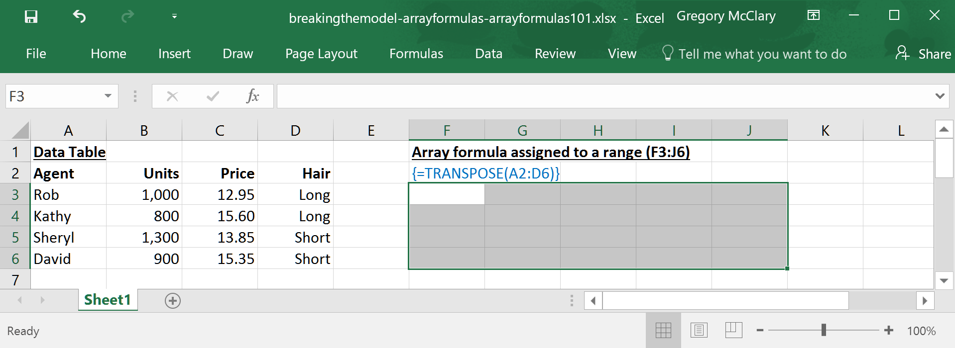
Next, type the array formula (do not type the braces {} – Excel will add these later). At this point, I’ll need to press ctrl-shift-enter to have Excel interpret the formula as an array formula.
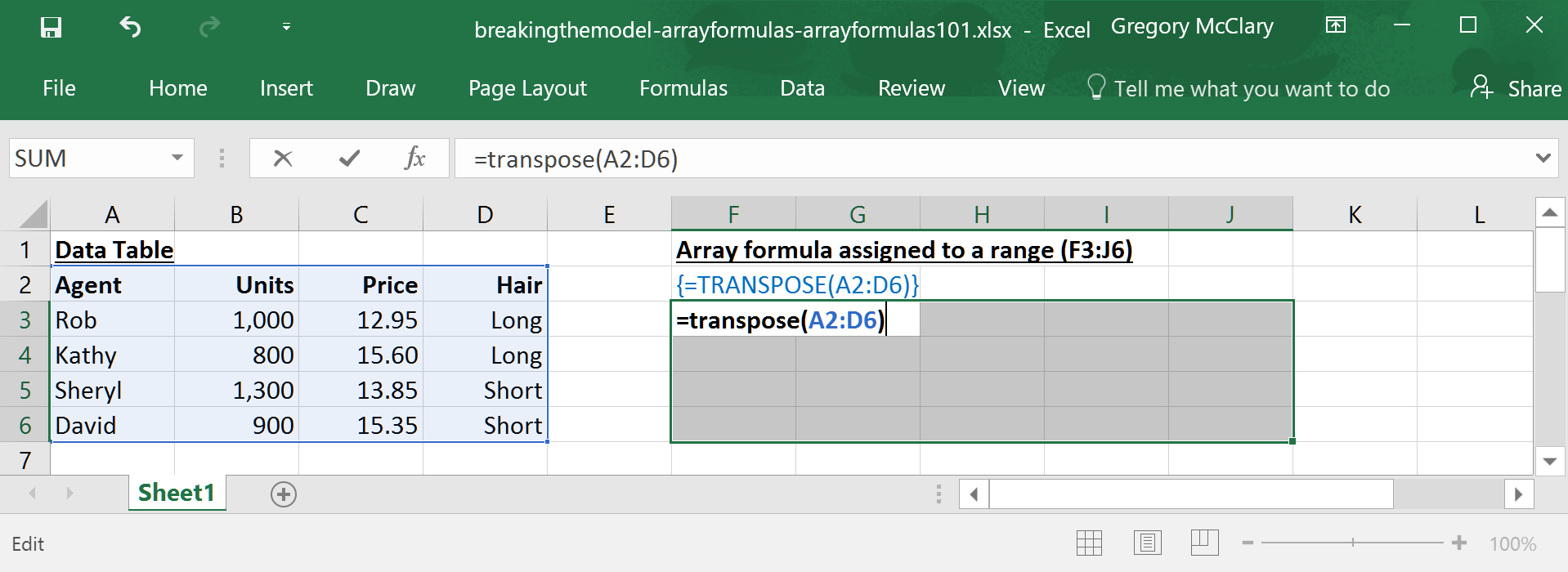
After pressing ctrl-shift-enter, Excel assigns the array formula to the selected range and displays the formula enclosed in braces {} in the formula bar.
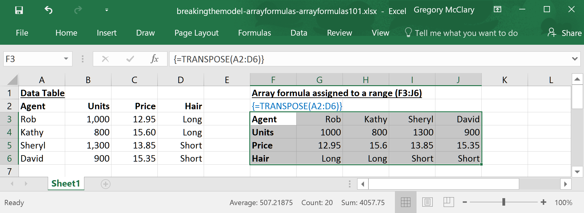
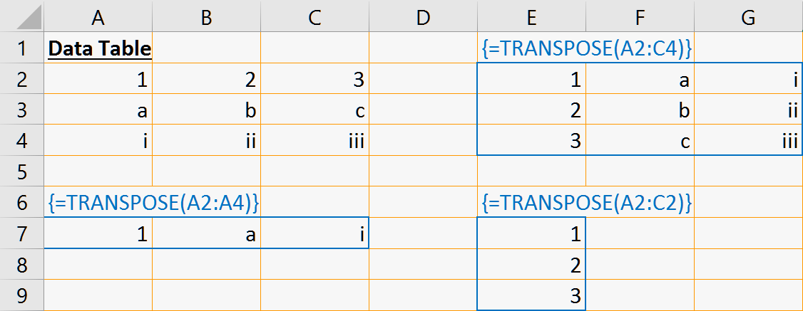
The example above makes use of the TRANSPOSE() function. Unlike most array formula-compatible functions, TRANSPOSE() only works in the context of array formulas. This formula performs exactly the same function as the “Paste Special…>Transpose” option, except that its output is responsive to changes in the source data. Click the button below for a complete rundown of the TRANSPOSE() function.
Returns a range of data with columns swapped for rows (a horizontal range would return in a vertical configuration)
The TRANSPOSE() function is almost useful enough in itself to make array formulas worth adopting, no? Let’s continue with a few more of the basics and make this thing bigger!
Lesson 2: Resizing and deleting array formulas
We’re almost through the dry stuff – this lesson has three key takeaways:
- You can only resize a multi-cell array formula to a larger range. To resize the output area, select the new area, click in the formula bar (as if to edit the formula), and then press ctrl-shift-enter.
- If you define an output range that exceeds the dimensions of the array formula’s output, Excel will report #N/A errors in the cells that are ‘out of range’.
- To define a smaller area, you actually need to select the entire range of the array formula, delete it, and either re-type or paste (you copied the formula before you deleted it, right?) the formula into a smaller range.
To expand an existing array formula, select a larger area that encloses the original array formula.
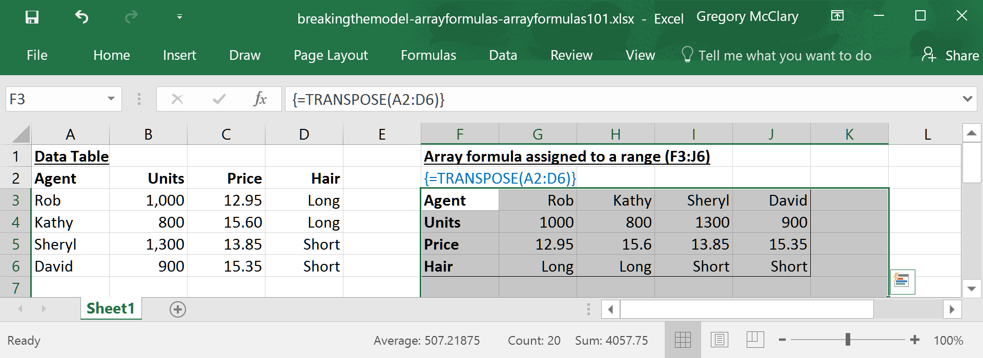
Click as though to edit the formula in the formula bar (but don’t change anything) and press ctrl-shift-enter.
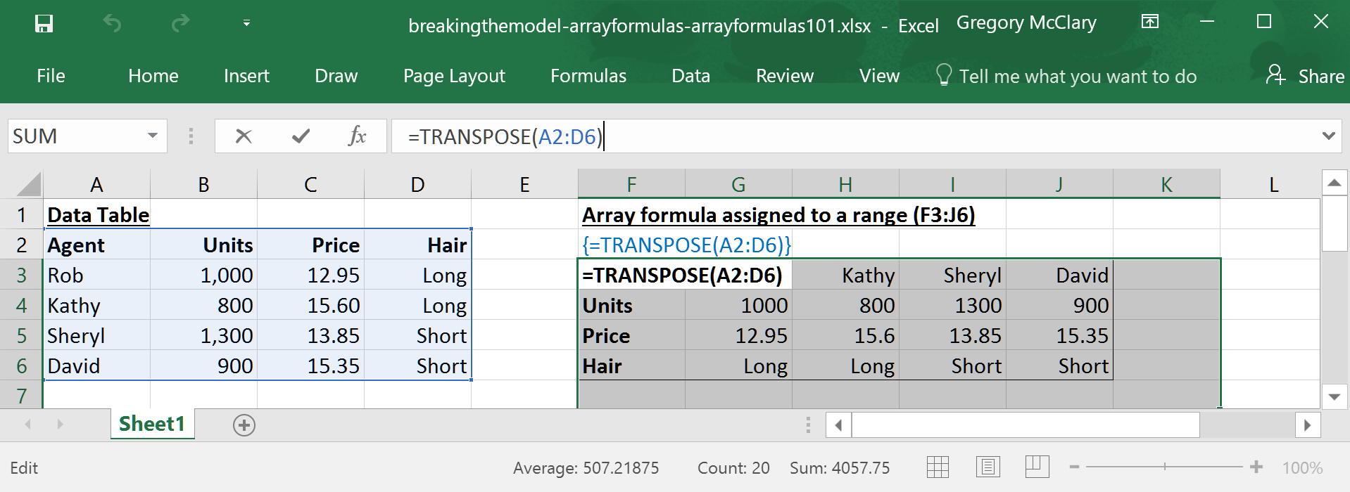
Once you’ve hit ctrl-shift-enter, you should see something like the screenshot below. Note that the array formula returns #N/A errors wherever the array formula’s output range exceeds the range that is returned from the array formula operation(s).
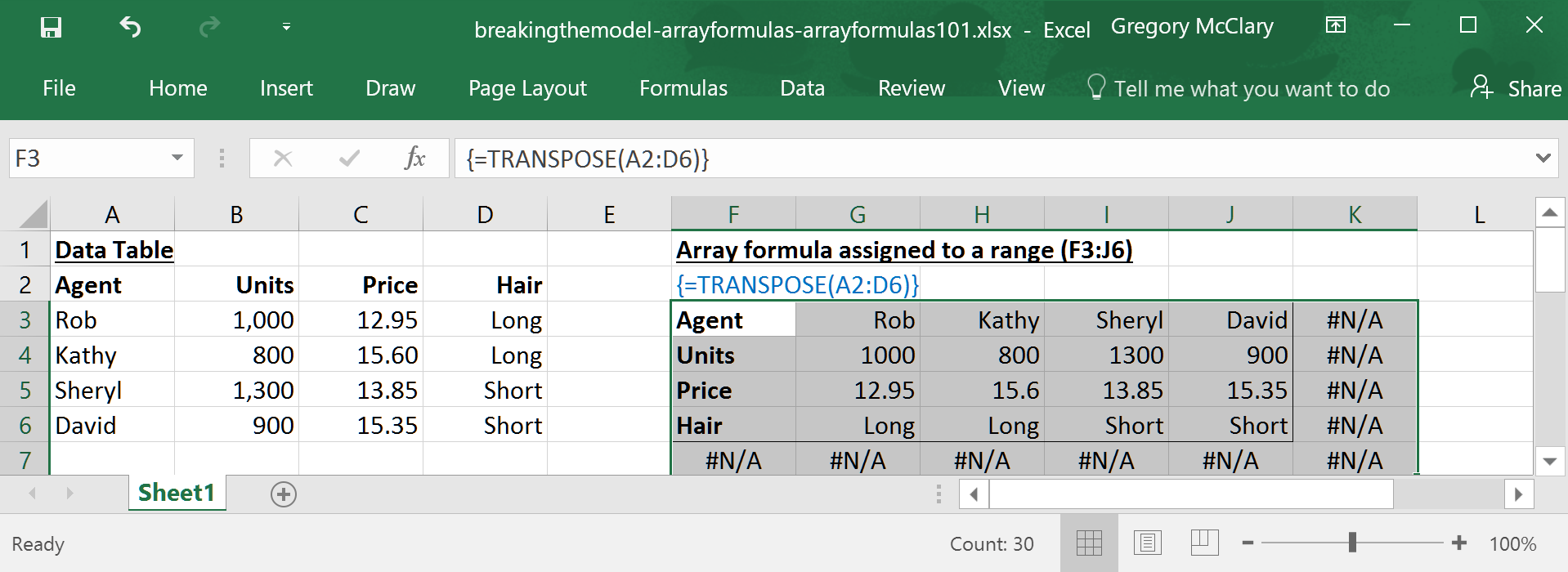
Realizing the error I made in the previous step, I selected the entire area enclosing the array formula and pressed delete. Array formulas cannot be resized into a smaller area, so I’ll need to repeat the process outlined in Lesson 1 (or press undo a couple of times…).
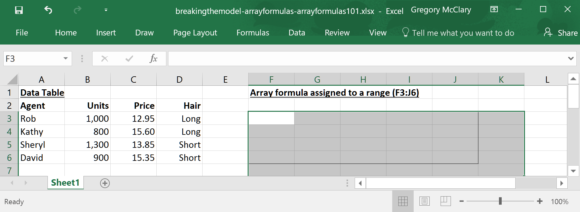
As these examples demonstrated, operations on ranges can be somewhat difficult to troubleshoot because any mismatch between the size of ranges can carry errors through into subsequent functions in the formula. This can be baffling (initially, at least), especially when your formula is returning a value to only one cell. It is important to visualize how arrays will be operated on as they flow through each operation and what data types each function or operation is going to return along the way.
Although it can take some time to grow comfortable working in this domain, array formulas allow you to perform complex calculations with ease once you’ve put a few notches in your belt. On that note, the button below gives a full rundown of the IF() function, which features prominently in the next few examples.
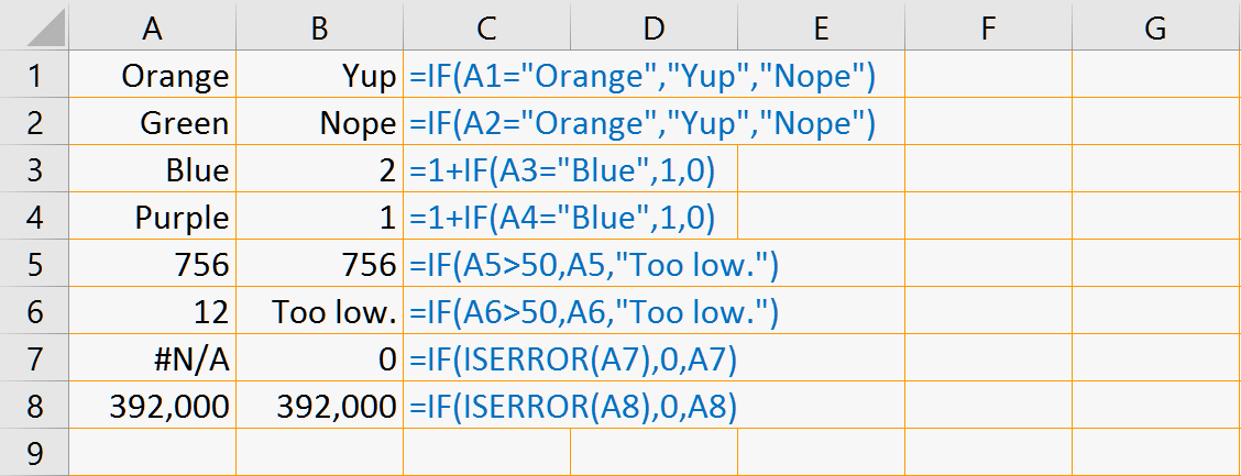
Returns one of two values or ranges of data depending on the outcome of a logical operation
Is this article ever dense, eh? Gratuitous digressions aside, let us direct our gaze to the main event:
Lesson 3: Adding functions and arithmetic to the mix
Now that you’ve seen the basics, lets check out the main attraction: operating on ranges.
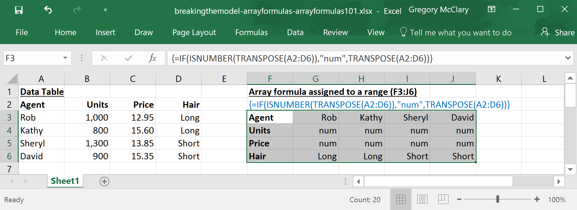
Let’s bring an IF() statement into the mix. This formula checks if the source data is a number (or a date); if yes, it will return “num”; if no, it will return the source data.
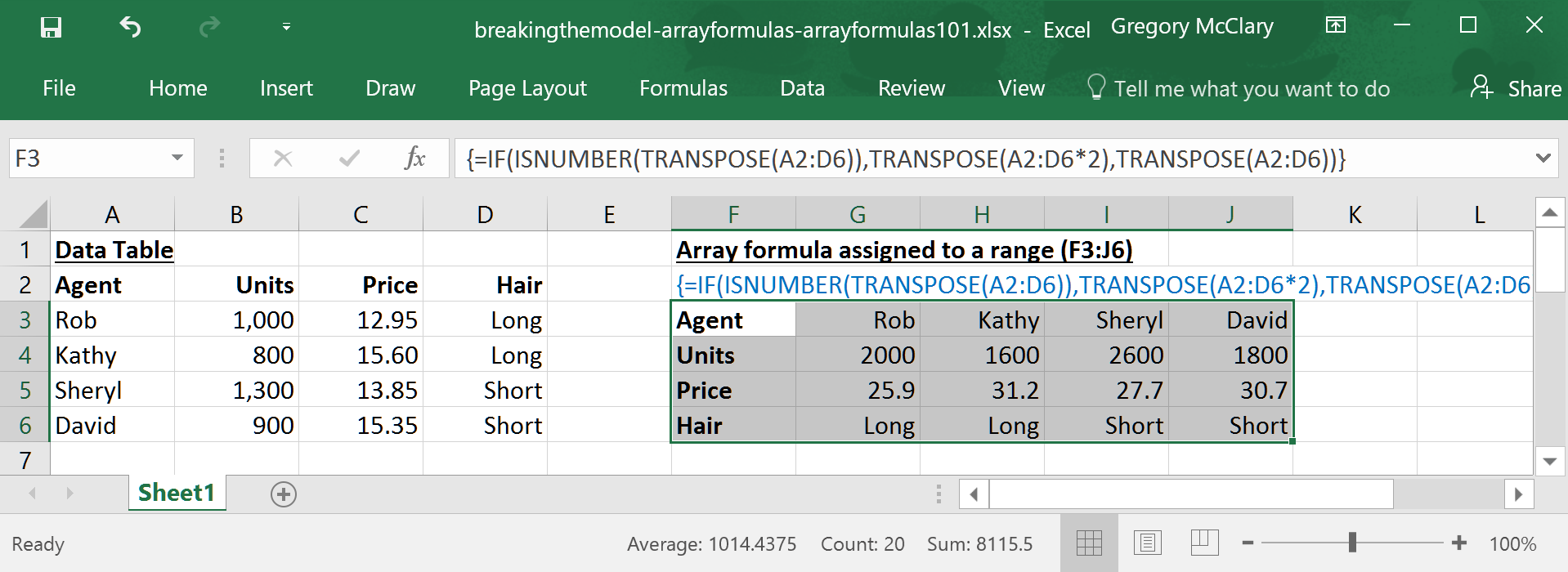
With a little tweak, instead of returning “num”, this formula will now calculate management’s sales targets for the team. It does this by multiplying each number in the target range by two. Twice the volume at twice the price equals pure profit, my friend.
And since it doesn’t matter if Excel transposes the data before or after it performs the IF() function, a more concise version of the last formula would look something like this:
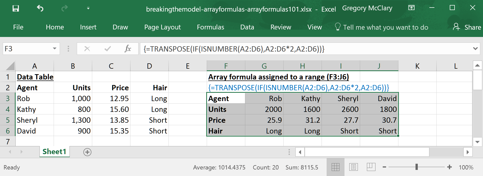
Although multi-cell formulas are somewhat cumbersome (particularly given the inability to downsize), this functionality is often a good way to troubleshoot the middle steps of a larger formula. As you construct array formulas, visualize what you would need to do to perform the same calculation in actual ranges. Keeping track of how the array is manipulated at each step of a calculation is the most important (and initially difficult) part of working with array formulas.
The real power of array formulas, however, is their ability to use native array formulas (like SUM(), AVERAGE(), CONCAT(), PERCENTILE(), etc.) to reduce operations on ranges into a single-cell array formula. This is where array formulas really excel – single-cell array formulas retain the ability to operate on ranges and allow you to calculate descriptive statistics on the results. Not only can this make it easier to analyze a data set, it will supercharge your ability to quickly and intuitively mine complex calculated values from any data source, on demand.
The next example uses SUM() to aggregate a calculation on a range into a single-cell result. Click the button below to launch a fulsome discourse on the subtleties of SUM().
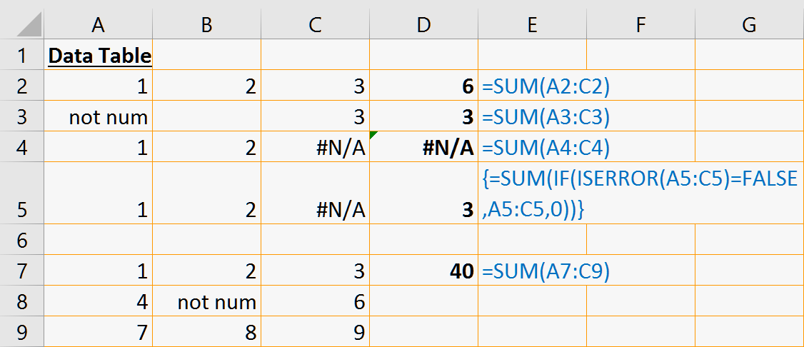
Returns the sum of all numerical values in one or more cells and/or ranges
The following example uses multi-cell array formulas to illustrate the intermediate steps calculated by the single-cell array formulas featured in the example.
Lesson 4: Introducing the single-cell array formula
Array formulas’ ability to output into a single cell is what makes this functionality so powerful. Instead of creating a full column to operate on, array formulas allow you to calculate an entire column worth of data and pass that on to another formula.
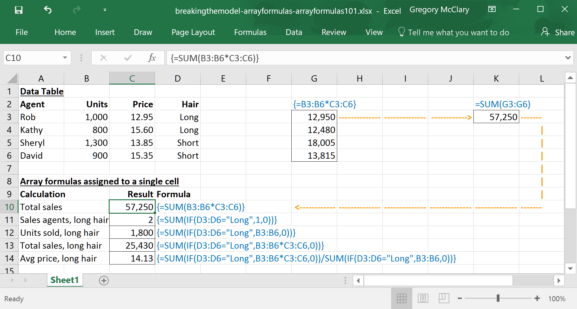
The only difference between inputting single- and multi-cell array formulas is whether you select one or multiple cells before you input the formula. Here, you can see that I’ve selected one cell, inputted my formula, and am poised to press ctrl-shift-enter.
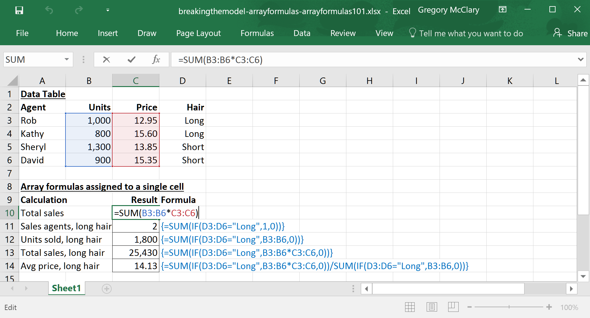
As noted above, the easiest way to get comfortable with the inner workings of array formulas is to visualize the arrays that are being passed through each function. in the screenshot below, I’ve separated each term in the formula to show what’s going on behind the scenes.
One feature you’ll notice about single-cell array formulas is that they tend to ‘finish’ with one of Excel’s native array formulas (like SUM(), AVERAGE(), CONCAT(), PERCENTILE(), etc.). These formulas all operate on an array to produce a single result, whether you’re using an array formula or not. As such, these functions are behaving exactly the way you would expect under normal Excel usage.
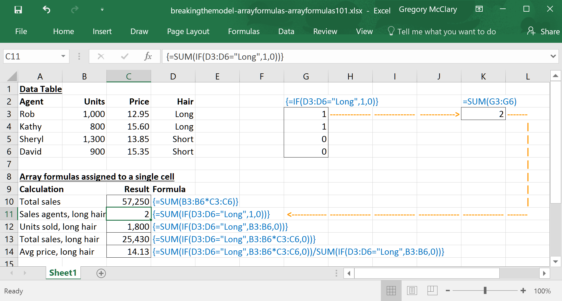
If you’re familiar with the formula, note that this particular array formula performs exactly the same function as the COUNTIF() function.
If it’s likely that you’re using many array formulas throughout an application, it can be more efficient to use array formulas even to perform calculations like this, where native array formulas are available for the same purpose – later, you’ll be able to copy-paste the logical operation in the IF() statement into other array formulas if you want to reuse the same logical filter again.
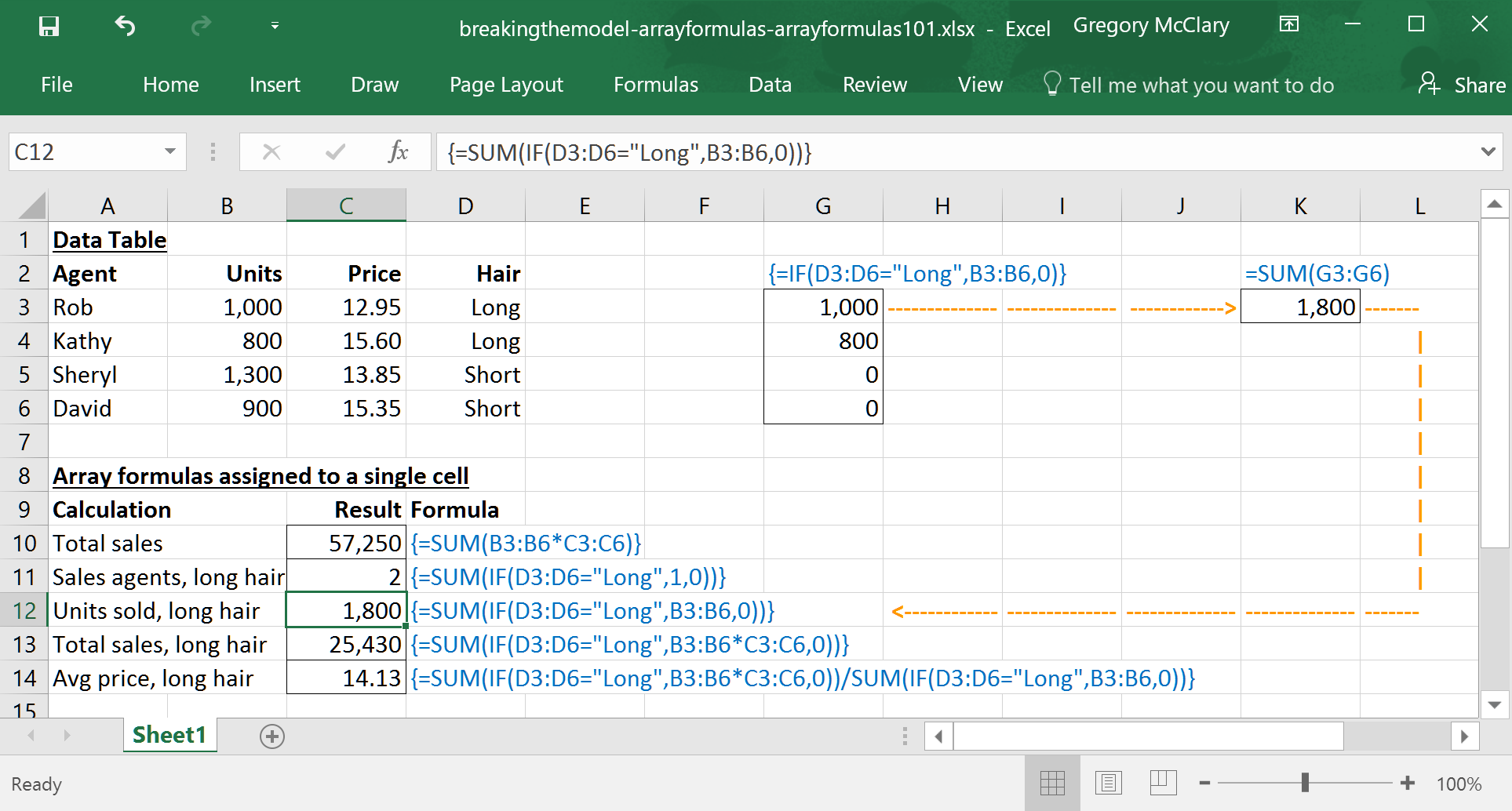
If instead of returning a count, I want the same formula to tell me total units sold for the group that we just counted, I can just change the value_if_true parameter in the IF() function to return the corresponding amount in the units column.
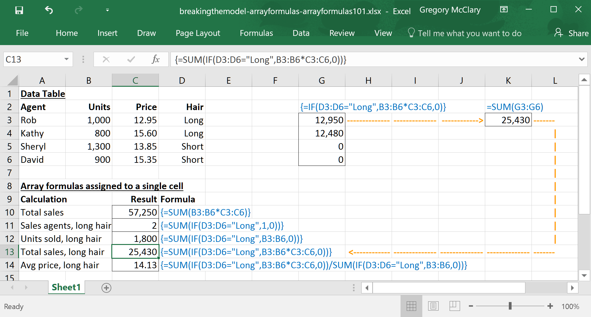
The next example adds arithmetic back into the mix. In order to calculate the total sales from long-haired salespeople, I need the IF() function to calculate the product of units and average price. A formula like this basically allows you to add a filter to a SUMPRODUCT().
The last example shows the compatibility of array formulas with the regular Excel environment. It is very important to note that array formulas allow you to do all of the things you would normally do in an Excel formula – the ability to operate on arrays just adds scope to what Excel will allow a formula to do.
Here, I have instructed Excel to calculate the average price of units sold by long-haired salespeople. This formula divides the formula that appears in the cell immediately above it by the complete formula one row above that. Even in an array formula, Excel just operates normally once it reaches the final calculation involving only single values.
Perhaps the biggest hurdle in learning to work with array formulas is building familiarity with how Excel passes data through these formulas. In particular, pay close attention to which functions/operations are passing either arrays or single values within a larger formula.
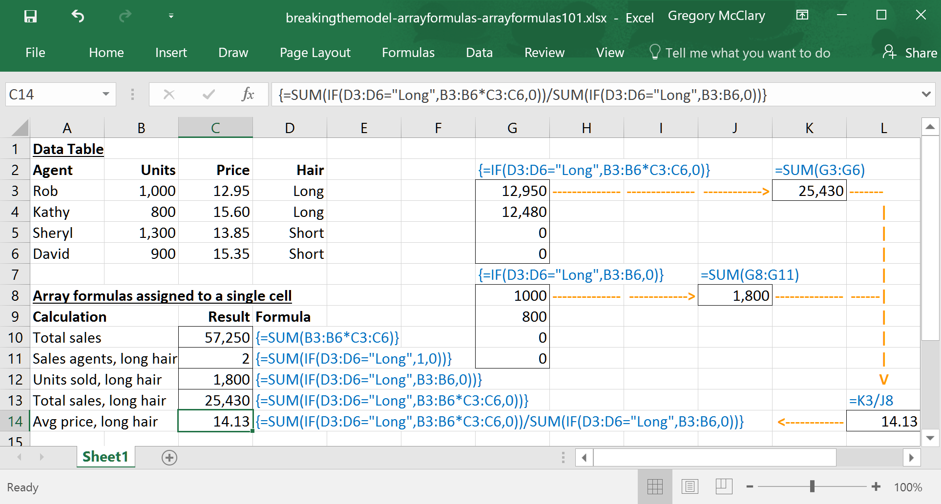
What this example illustrates is that array formulas can be used to perform pretty much any bulk calculation that you can dream up – without resorting to pivot tables (which might involve calculated fields, etc.) or other unwieldy solutions. In practice, this concept is expansive – and now, we enter the rabbit hole.
Although it takes a bit more effort to grow comfortable with array formulas, using them to perform compound calculations on ranges can save you a lot of time and stave off a good amount of clutter in your spreadsheet. This lesson shows the use of powerful (yet reasonably simple) array formulas doing a few things that would be cumbersome to perform step by step.
Before you jump in, check out AVERAGE() and PERCENTILE(), if you’re not already hip to the scene (or you just enjoy the sleek animation of modal popups on this site).
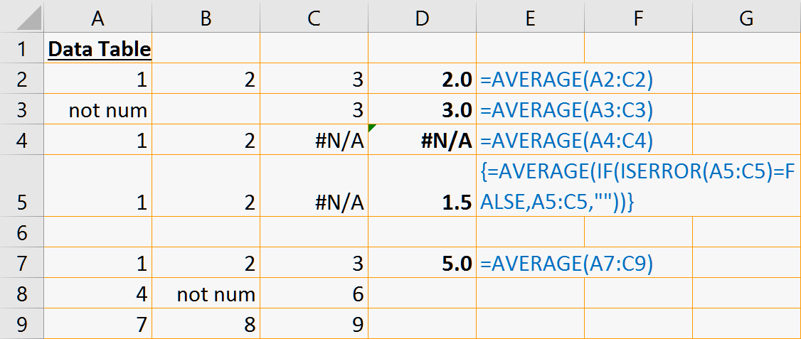
Returns the arithmetic mean of all numerical values in one or more cells and/or ranges
Returns the nth percentile of values in a range
Moving right along, then:
Lesson 5: The all-powerful single-cell array formula
The following example shows how single-cell array formulas might fit into something that looks more like a real-world analysis. In this example, I’ve set up each formula such that it references only the data table on the left to demonstrate the array formula’s power in this respect. Notice how array formulas allow us to get much deeper into an analysis than Excel’s normal environment would permit in a single cell.
Click the toggles below for a blow-by-blow explanation of the array formulas used in this example.
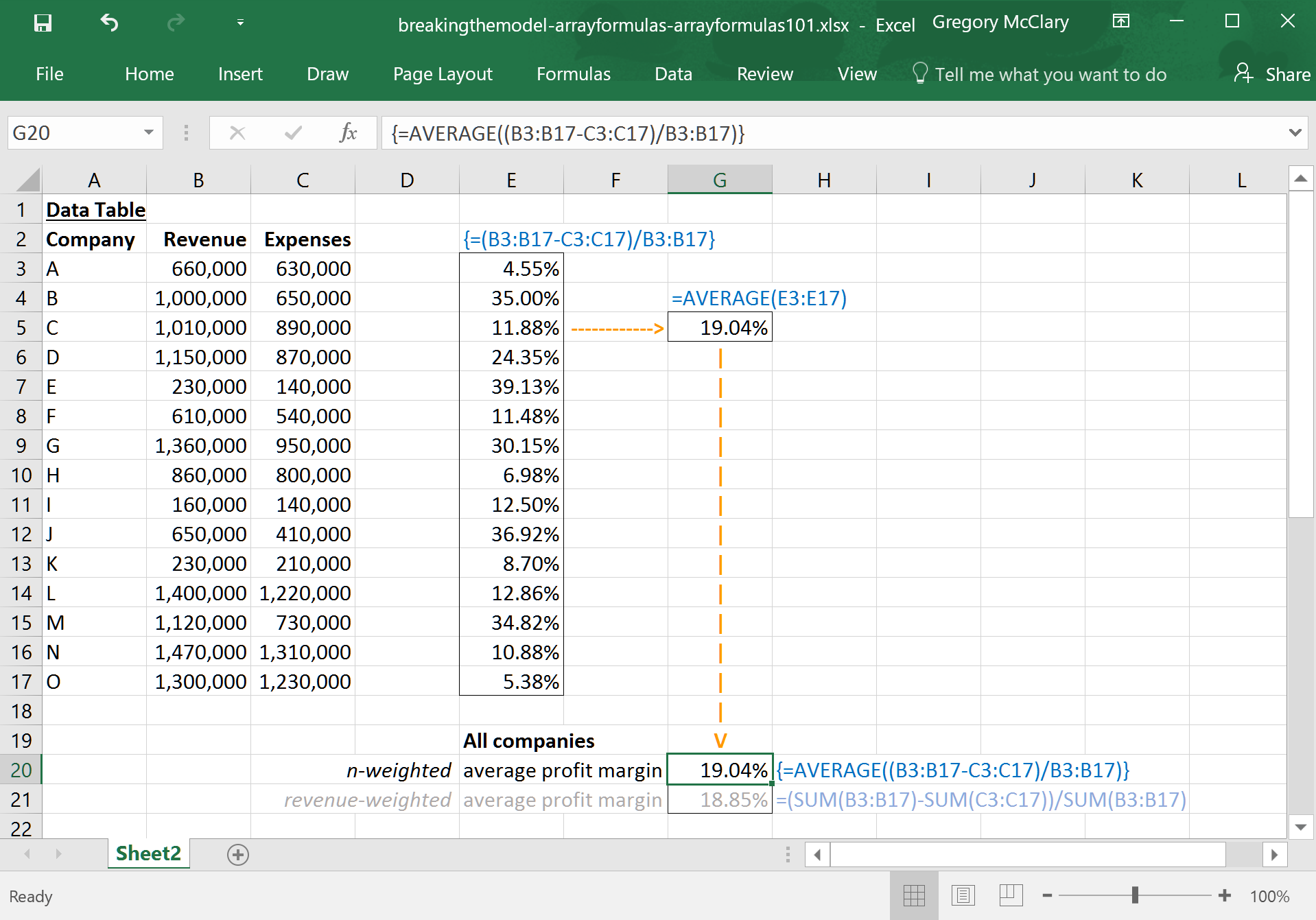
The first calculation that required an array formula was ‘average profit margin’. For whatever reason, I wanted to calculate an n-weighted average profit margin for the entire sample. In other words, I wanted to take the average of profit margins of companies irrespective of their revenue (as opposed to the revenue-weighted average which I’ve also begrudgingly calculated in the screenshot below).
To perform this operation, I needed a list of profit margins of which to take the average. The expression inside the AVERAGE() function does exactly this; it performs the (rev-exp)/rev operation all the way down the column and outputs the single column result to AVERAGE(). AVERAGE() then returns the mean using this list of calculated values.
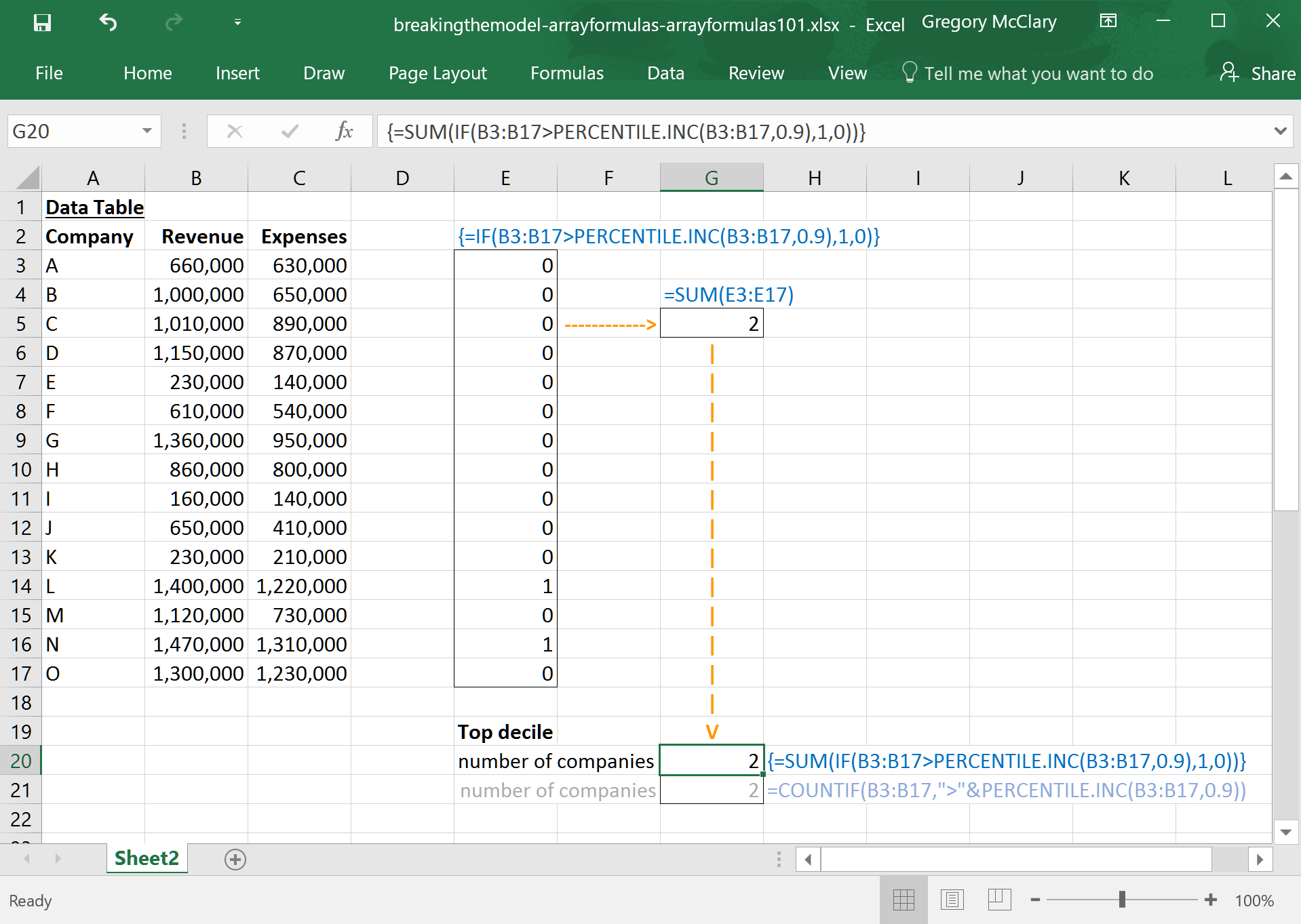
By row 11, the analysis again requires an array formula. Here, I used the formula on row 10 as one of the terms in the logical_test in the IF() statement. Altogether, this logical_test acts as a filter for companies with revenues exceeding the top decile threshold for revenue; if yes, the IF() function returns 1; if no, it returns 0.
This array formula performs essentially the same function as Excel’s COUNTIF() function (as illustrated in the lighter shade of text below). As a rule, I’m not a fan of formulas like COUNTIF() that take logical arguments as a string. In this case, using COUNTIF() requires us to use an ‘&’ operator to incorporate PERCENTILE() into a text-format version of the logical operation. The virtue of using the array formula version instead of COUNTIF() is that we will be able to reuse most of what we’ve already typed for the current formula when we move on to the next one.
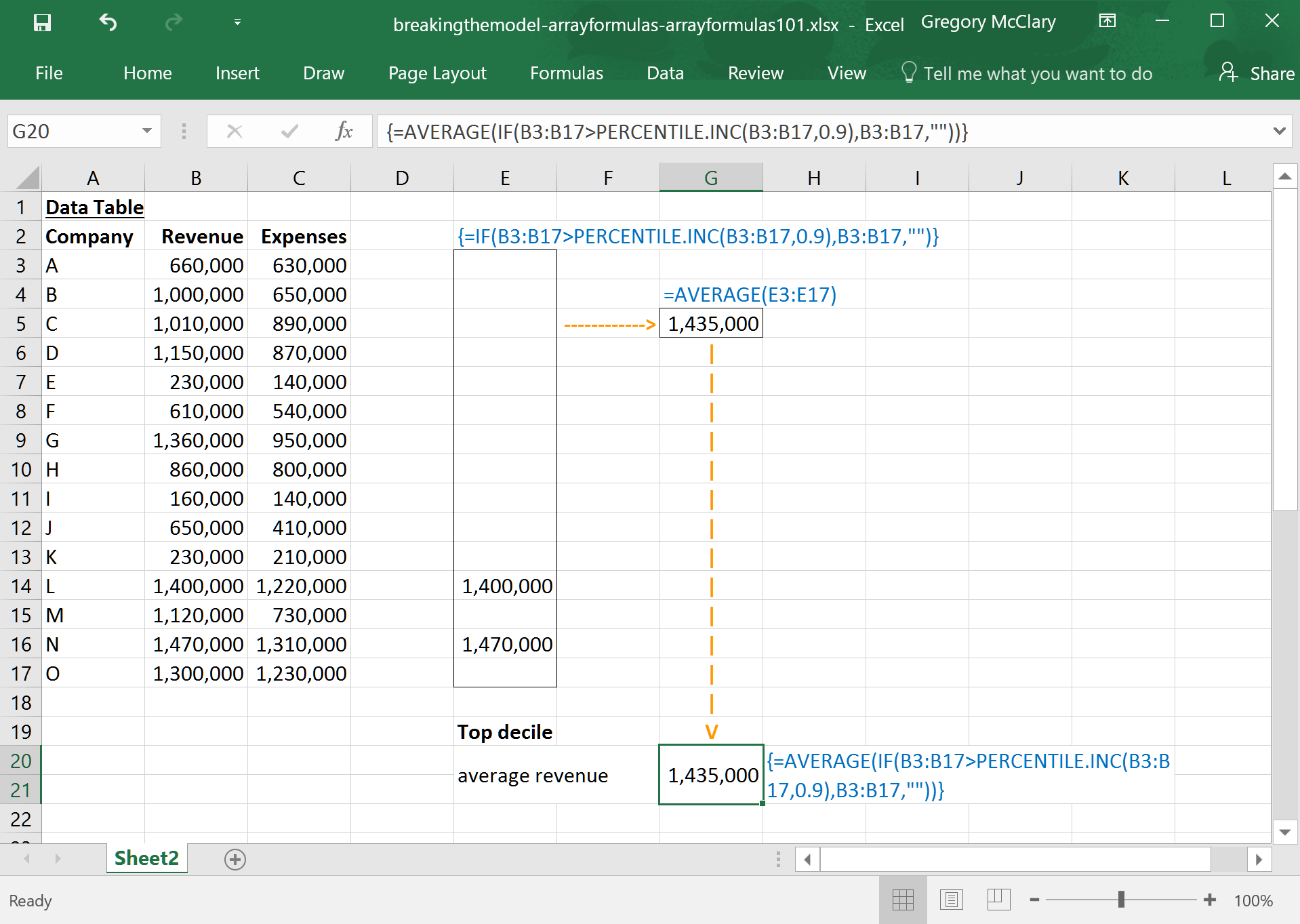
The formula in row 13 uses the same logical_test filter mentioned in the last step. In this instance, however, the IF() statement returns either: company revenue; or “” (because AVERAGE() does not operate on non-numerical values – convenient, no?). AVERAGE() then simply computes the mean of any revenues that made it onto the list.
An identical operation was applied to expenses in the formula below average revenues (row 14).
In the final calculation of the example, I decided to compute the n-weighted average profitability of companies in the top decile. Here, the IF() statement populates a list containing the profit margin for qualifying companies. Once again, for companies that are not in the top decile, it adds “” to the list to ‘hide’ these entries from AVERAGE(). Finally, the AVERAGE() function computes the mean of profit margins in the list and returns a single value, as expected.
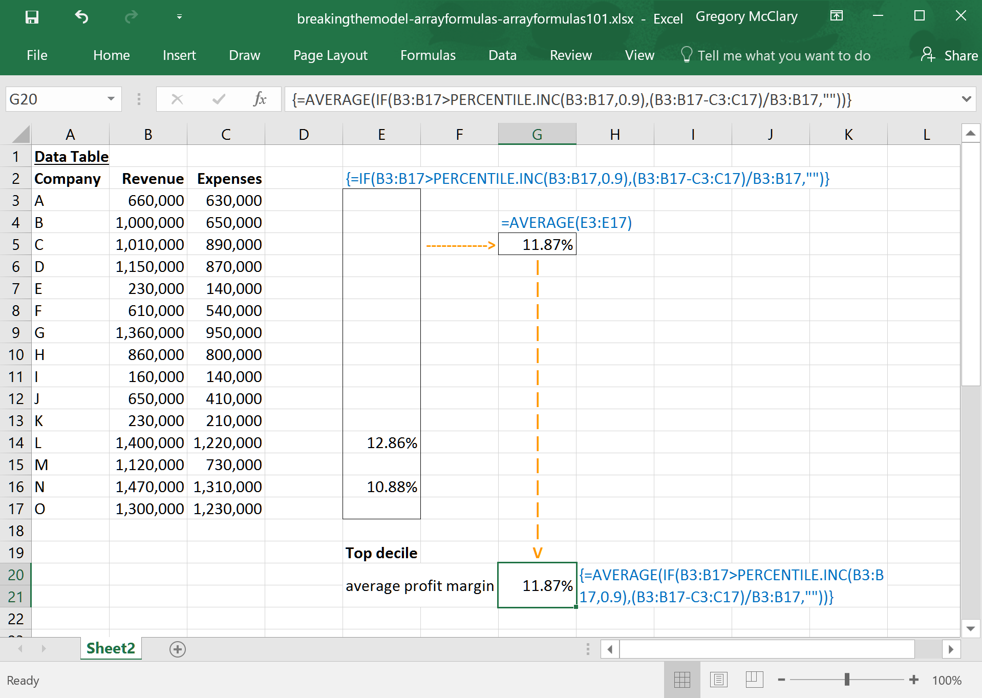
More generally, it is important to note that some array inputs are handled differently depending on which formula is operating on them. In the last formula above (row 16), the PERCENTILE() function operates on a range and then returns a single value. This single value is then compared against each term on the other side of the logical operator ‘>’.
It is tempting (but incorrect) to worry that PERCENTILE() could interpret this formula such that it iterates through the range and returns an array with a separate percentile calculation for each individual value in the range. Fortunately, Excel handles arrays systematically (at least among the functions that are available to use in array formulas – more on that later).
The key difference here is that the IF() statement receives a single value output from PERCENTILE() – because that’s exactly what the PERCENTILE() function always does when it operates on an array – and then compares it to each value in a range. As a result, the formula compares each revenue data point to a single value. It is also possible to compare two lists item for item – you would just need to specify an array for both sides of the logical operator (or use functions that return arrays).
Epilogue
Although there’s a bit of a learning curve, array formulas are blindingly awesome if you happen to spend some (or all) of your days entangled in webs of gridlines. I hope this installment encourages you to dig deeper. Stay tuned for the (forthcoming) second installment of this series, Array Formulas 201.
Array formulas add new dimensions to your equations – the first and second dimensions, to be precise
Subsequent installments in this series will help you put array formulas to work effectively, and develop broader Excel habits that will streamline your overall workflow as you cut your teeth with this versatile toolkit.


