Broad Strokes
Array formulas you will actually use
So – here you are. The evidence suggests that you’re now convinced of array formulas’ awesomeness. As noted (repeatedly?) in the previous article, one of my biggest grievances in life is the apparent non-existence of documentation about array formulas. My goal in authoring this series is to make this rather opaque toolkit more accessible. In that spirit, this article (and the one that follows) will thoroughly work through several practical uses for array formulas while also highlighting useful style considerations. Although the first installment of this series really highlights the power of this domain, there are some (honestly, many) quirks that litter the landscape. This article also pours a technical foundation that is invaluable in the context of troubleshooting.
While there is no ‘right’ way to do anything in Excel, the use of array formulas presents some opportunities that may not be immediately apparent. As such, Array Formulas 201 focuses on applying these formulas to the type of task in which their efficiency really shines. More specifically, the topics addressed in this installment include: tables in Excel (save your sanity – meet your array formula’s best friend), data filtering, compound logical operations in the array formula environment (e.g., AND() and OR()), lookups, and cross-tabulation. In doing so, it also presents a sensible framework with which to organize this particular type of analysis. Possibly the single least documented aspect of using array formulas is how to organize the dense swaths of summary statistics that array formulas so excel at producing.
For the keeners, the following article, Array Formulas 301, will tackle more advanced and/or specialized use cases such as lookups on two-dimensional ranges, compound formulas, sorting, and semi-intelligent, large-scale error handling/sumchecks. In sum, the material covered in this article will arm you with (almost) everything you will need to begin employing array formulas in a variety of real-world situations, whereas the next dives into the design of more complicated compound formulas, streamlining the reporting process, and ensuring data integrity in your work.
Usage and Style
Employing array formulas flexibly will empower your intuition;
however, with great power comes great responsibility
As you begin to apply array formulas in your day-to-day, you will soon find that there are a ridiculous number of ways to construct any given analysis. This article will not only celebrate that freedom, but also address the practical imperative of making your work both transparent and easily editable. It is not raw speed that makes a great Formula One driver – rather, it is disciplined pacing, effective manoeuvering within the pack, and grace through corners. So too with great Excel formula designers – developing and adhering to a coherent stylistic framework will ensure that you more quickly reap the time-savings and flexibility that array formulas avail.

Thoughtful, Disciplined Pacing
As you see more and more uses for array formulas, you will find that not only organization, but scalability and editability begins to dominate your thoughts. By spending a little extra time on the front end, you can ensure that the work you do now will be easy to parse and/or reuse in other analytical contexts. While array formulas can save oodles of time overall, they do this best if you apply a little more attention to flexibility in the design phase.

Manoeuvring Within the Pack
Not only should you be concerned with your own capacity to parse your work, you may be passing this work on to others. The more your work follows a consistent and logical flow, the less critical it becomes for downstream users to be familiar with array formulas themselves. Additionally, the metaphorical ‘pack’ may call for changes in your work – good Excel style will allow you to quickly and transparently accommodate such requests.

Grace Through Corners
I don’t hear the word agility used very often in describing an analysis, but I suspect that the best analyses are those in which the analyst has the capacity to quickly and easily test ad hoc hypotheses along the way. I’ll never find a relationship that I don’t test, and I’m much less likely to test a low-conviction hypothesis if it will take hours to run with it. Employing array formulas flexibly will empower your intuition.
If you’re not already driving Formula One cars down ski hills,
I suggest you start today.
One thing you will immediately notice about using array formulas is that it drastically changes the way that you interact with Excel. When you might previously have jumped back and forth between sheets, pulled up dialog boxes, manually manipulated data, or ran through a sequence of tables, you will now spend your time thinking about the logical basis on which to automate a task, how you can best organize your analysis, and by what means you can ensure that all of your formulas performed operations in the way that you intended. This article will faithfully address the spatial and organizational implications of using array formulas effectively in real-world applications and introduce the thorough (and very necessary) application of sumchecks.
As a word of advice, keep track of how much time you would have spent performing a task by other means and compare the result to your performance with the use of array formulas. My experience is of getting noticeably faster as I become more adept at recognising opportunities to mine data more efficiently and intuitively.
The Good Stuff
Tables in Excel: not redundant!
One thing I really like about pivot tables is that the interface uses text in the column heading to reference entire columns of data. Likewise, tables in Excel allow you to reference entire columns of data in formulas using a table name and column heading. When you’re working with relatively complex formulas operating on ranges of data (array formulas, perhaps?), you can make them easier to interpret by using descriptively named references. They also allow you to actually see the data that is included (and excluded) by all formulas that reference the same source data.
For the purposes of this article, I’ve prepared a fake data set that will be referenced in all examples and formatted it as a table. This is the kind of data you might encounter after performing a survey of companies to facilitate a regional industry profile. There is a download link immediately below the following spreadsheet. You are warmly invited to click it.
Lesson 1: Working with tables in Excel
Working with tables is pretty intuitive, but it requires a bit of an orientation for the uninitiated. Click through the following toggles to learn how to insert, name, resize, and reference data in a table.
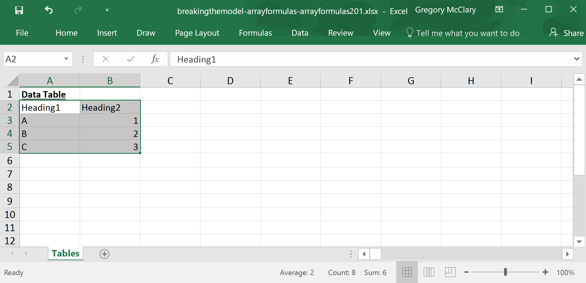
To create a table, first select a range containing the data that you want to include in the table.
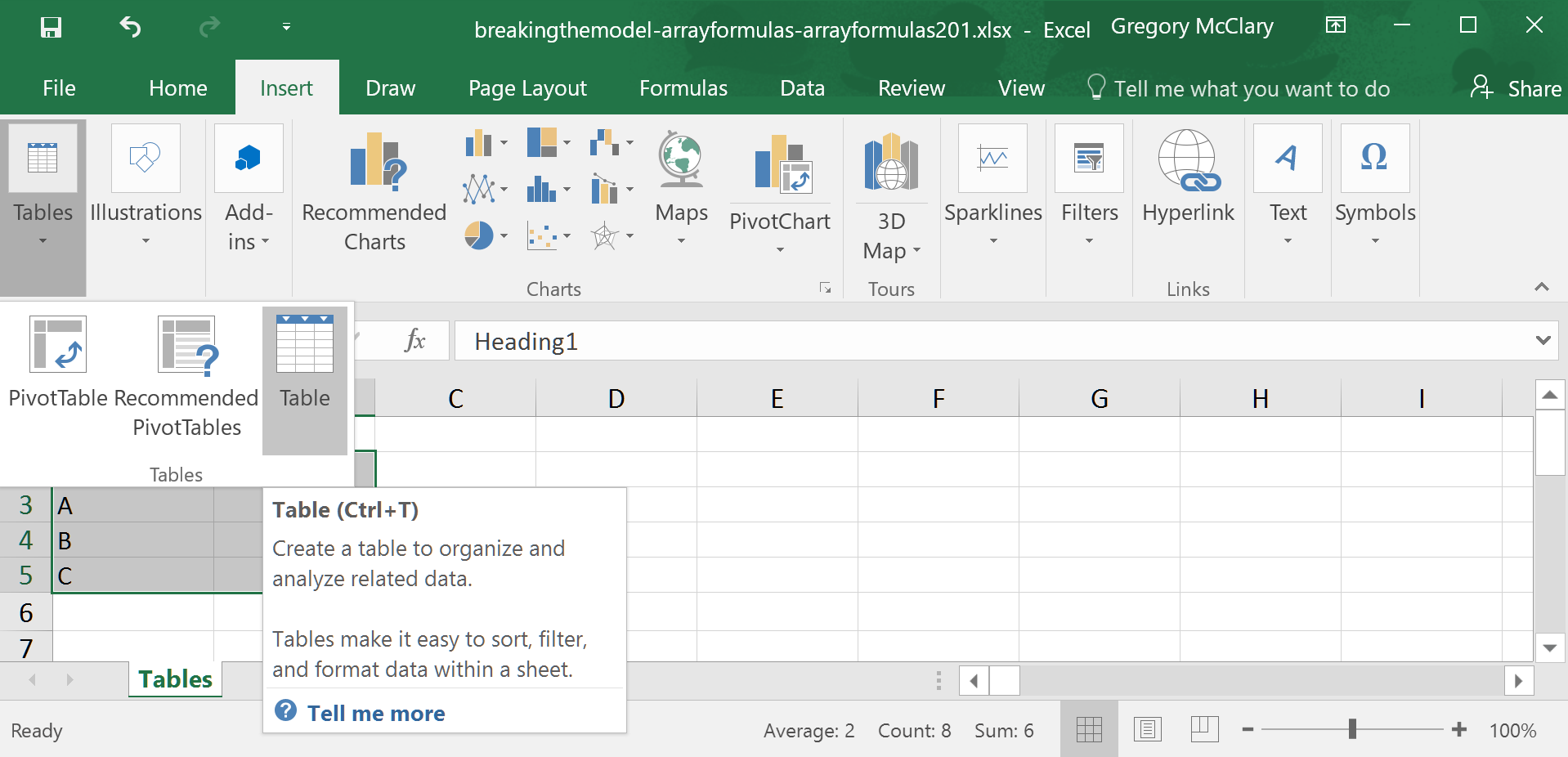
…or press ctrl-T. If you’re a Mac user, this keyboard shortcut won’t work. This key combination is configured to toggle between absolute and relative cell references by default on Office for Mac.
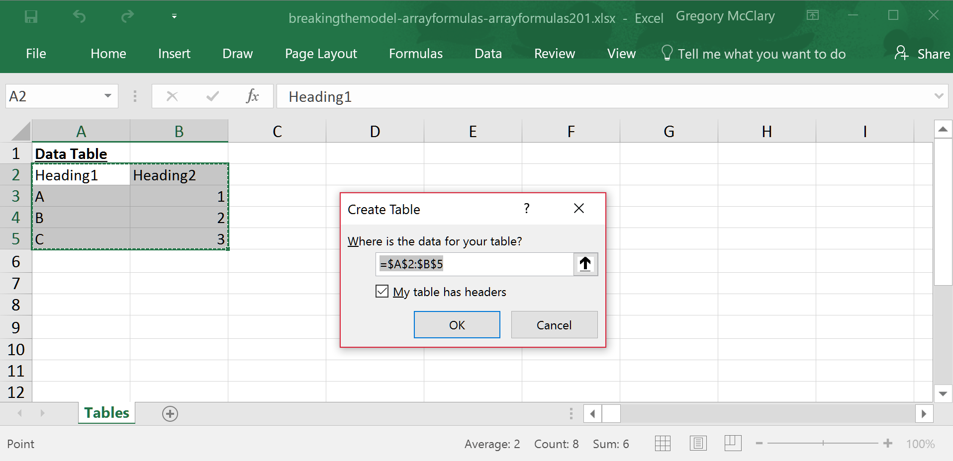
Since Excel was kind enough to bring up the topic of headers (via the checkbox below), I’ll note at this point that tables require you to use unique text column headings, as Excel will be using these to reference ranges of data within the table.
If you select a cell within the table, Excel will allow you to access the Table Design tab in the ribbon. Here you will find a field (on the top left) where you can type a customized table name. Remember that the point of all this is to make data easier to reference in formulas, so try to use the minimum number of characters that are adequately descriptive.
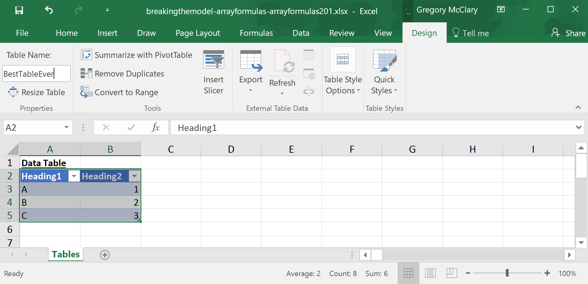
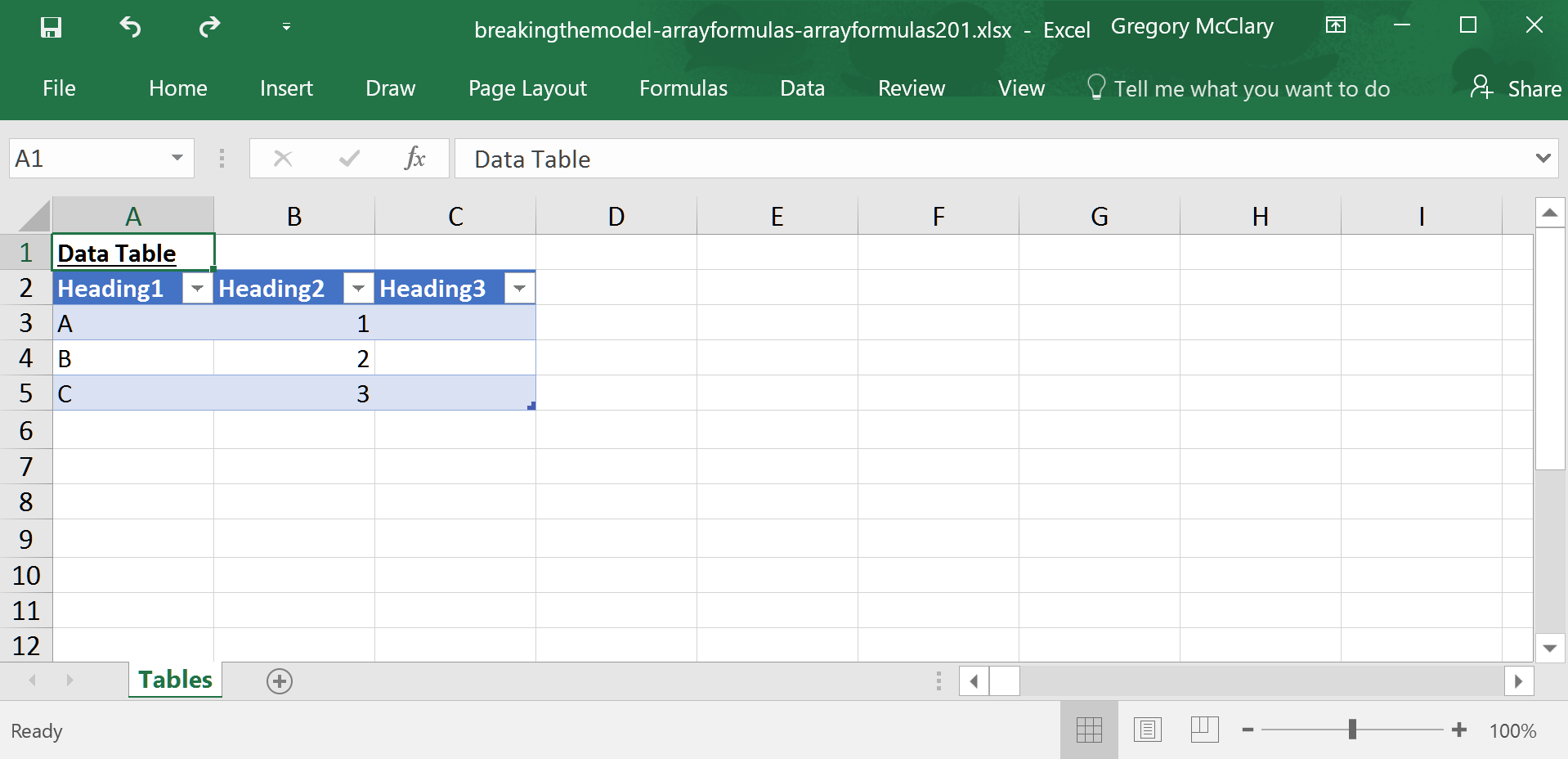
If you need to add a row or a column, Excel will automatically expand the table’s range if you type data into a cell adjacent to the table’s current range. Alternatively, you can click and drag the little blue tab that lives just inside the bottom right corner of the table.
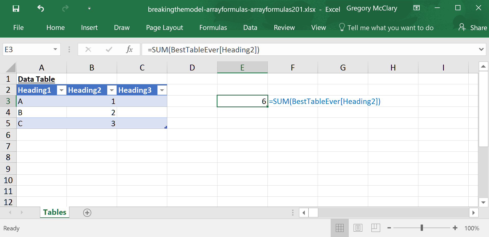
Now, you can easily reference the data in any column (TableName[ColumnName]), just the headers (TableName[#Headers]), all data in the body of the table (TableName), or the entire table including headers (TableName[#All]), and much more, all from the comfort of your friendly neighbourhood formula bar.
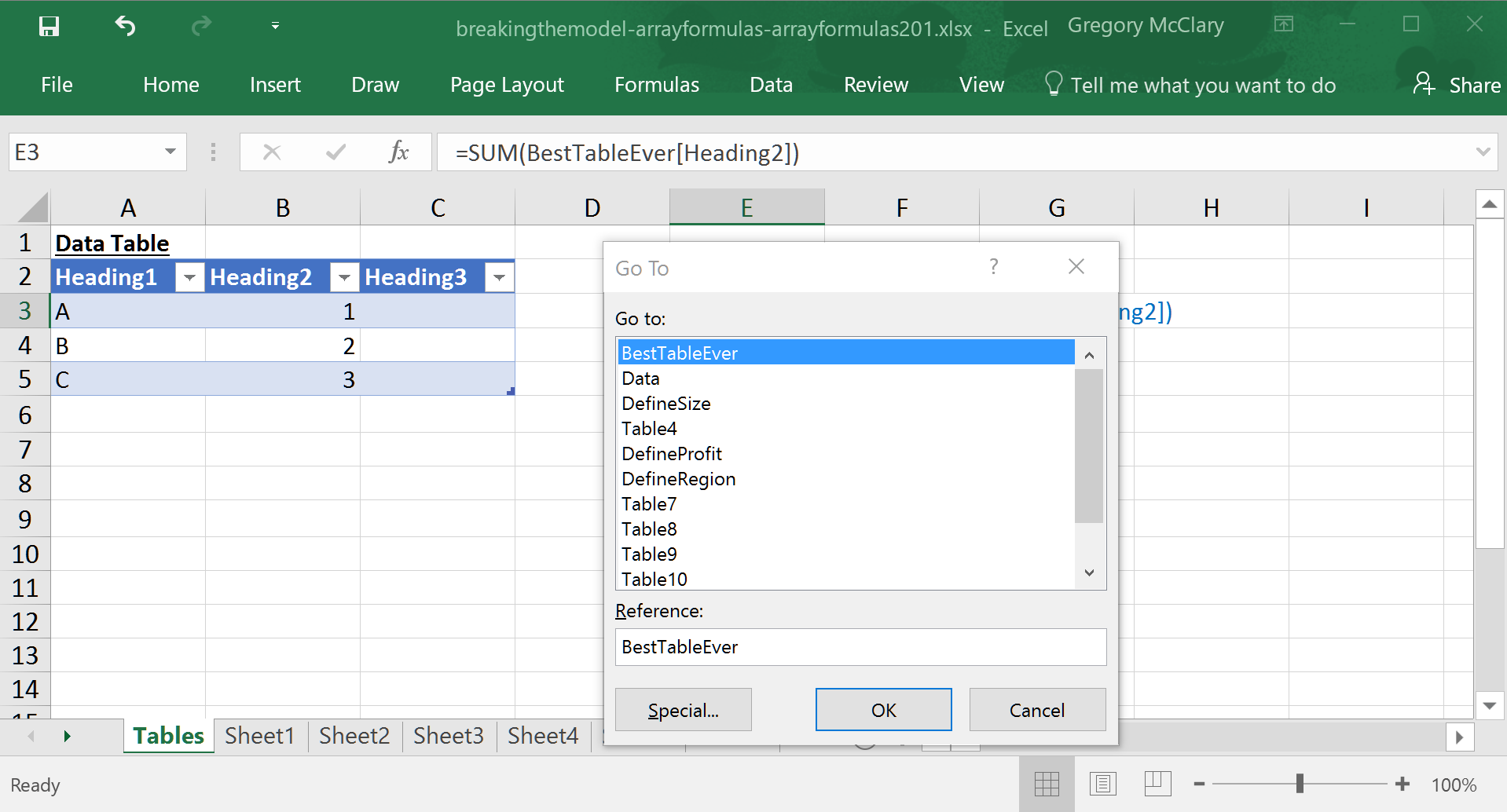
And one final, very useful, tip – tables obviate the need to reference the worksheet on which the table is located. This is a great feature to make your formulas cleaner, but it can be jarring the first time you ‘lose’ a table on a distant sheet.
If you press F5, it brings up Excel’s “Go To” dialog box. Here, you will see a list of every table in your workbook. Simply select the name of a table and click OK to navigate directly there.
As a final note, tables can do a lot more than just beautify your formulas, but it’s about time we turn back to the main event.
Before we jump into the deep end, I’d like to spend a few minutes to lay out the gritty details of how Excel interprets mathematical operations in array formulas. If you’re new to array formulas the following ‘rules’ will significantly reduce the break-in period:
If you specify an operation between two ranges, Excel will perform the operation between each cell and its similarly positioned counterpart in the other range. The operation will return an array (an imaginary ‘range’ populated by the calculated values).
If you specify an operation between a range and a single value, Excel will perform the operation such that the single value operates against each value in the range. The operation will return an array.
If you specify an operation between two single values (even in an array formula), Excel will return the single value result of the operation.
The first point above deserves some special attention; remember what we learned in Lesson 2 of Array Formulas 101 – if Excel runs out of ‘similarly positioned cells’ in one of the ranges that you specify, it will keep performing that operation through each cell of the larger range against the #N/A errors that Excel assumes to occupy any cell outside of the bounds of a range reference. If you are using a single-cell array formula, this error (likely plural) will carry through into the single-cell result (unless you deliberately set up a mechanism to catch/bypass errors).
Incidentally, these rules hold true for most functions as well. If a function is not able to return an array (and sadly, there are many that don’t, such as AND(), OR(), VLOOKUP(), and INDEX(), for example) it will return a single value. This outcome can be confusing because that single value will carry through the rest of the formula as outlined above. When you’re honeymooning with array formulas, you’ll soon learn that one of the most reliable aspects of array formulas is that mathematical operations, at least, always operate on ranges subject to the rules above. Functions… are hit and miss.
Since we’ve been taking it easy so far, the following lesson gives a leisurely illustration of how it will look when you start using tables to reference ranges with some mathematical operations in the equation (literally). After that, we’ll launch into the legitimately fun stuff.
Lesson 2: A leisurely illustration of mathematical operations and table references in array formulas
This lesson will be short and sweet, but I think it’s important to drive home everything that this article has touched on thus far. This is consistent with this site’s broader philosophy of allocating time to automate as much of life as possible.
In particular, note that the use of tables ensures that any two ranges (from the same table, at least) will be the same size. It’s simple to implement, and over the long haul, this practice significantly reduces the scope of troubleshooting you will need to conduct if a single-cell array formula goes bad (think #N/A).
Check out the screenshot below and click the toggles to accompany that exercise with some semblance of purpose.
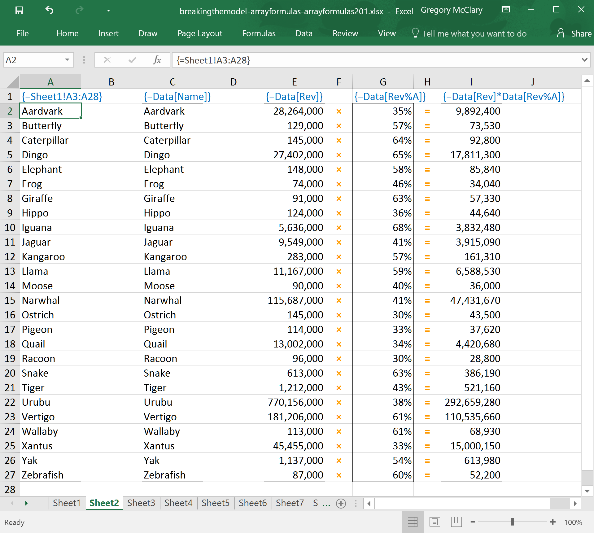
The formula in column A is obnoxious to type. I have to either navigate to Sheet1 and manually select the range, or conform to Excel’s convoluted reference naming conventions (that is, if I’m lucky enough to remember the column letter where my data is located).
With a table reference, as illustrated in column C, I can get the same result with less typing and I’ll have a better idea of what I’m looking at when I revisit the formula later.
The formulas in columns E and G show what Excel sees when you specify two different ranges. The orange operators show how Excel conducts the operation between two ranges when you specify the formula in column I. As noted in the text preceding this screenshot, remember: one of the most compelling reasons to use tables in conjunction with array formulas is that they will prevent you from accidentally specifying an operation between ranges of different sizes because each of the columns in a table will have identical dimensions.
I highly recommend playing around with operations on ranges of different sizes until you’re comfortable with their behaviour and where errors occur – that (moderately boring) exercise will make you considerably more efficient at troubleshooting errors returned by a single-cell array formulas.
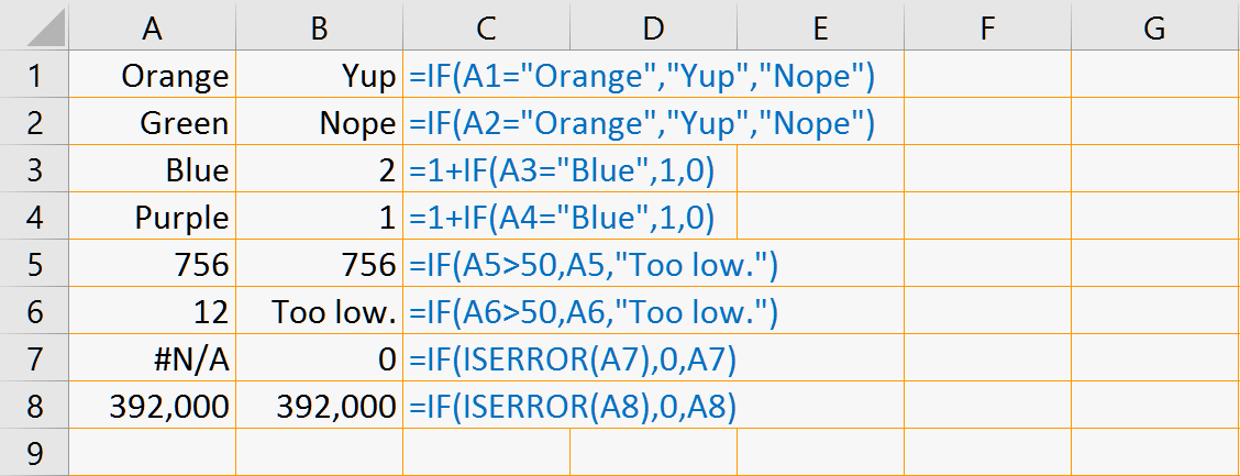
When working with databases, one of the most common functions you’re likely to use in your array formulas is the IF() function. This function allows you to control the flow of data through an operation based on one or more logical conditions. If you:
- skipped the first installment of this series and you’re not yet feeling nauseous,
- you read the first installment but skipped the modal popup about IF(), or
- you forget already,
you should probably click the button below and prepare to develop a fulsome appreciation of Excel’s shortest (and possibly most versatile) function.
Returns one of two values or ranges of data depending on the outcome of a logical operation
As some of the examples in the previous article showed, the IF() function can be used to act as a filter that passes selected data on to another formula. This is particularly handy when used in combination with statistical, mathematical and text functions that return a single value based on a range.
Lesson 3: Filtering data with IF()
IF() will let you selectively pass data on to other functions or operations. The remainder of this article will lay out various ways that you can exploit this capability to maximum advantage in your day-to-day analytical drudgery.
Before you scroll any farther, don’t forget to download the workbook from the link a little way back. Screenshots of a full 28 rows are awkward and I’m just not willing to go down that road (or I guess not as toggle box content, anyway).
So I was using Excel in French mode today (if you can really call it that…) and it seemed fitting to give Quebec a little love.
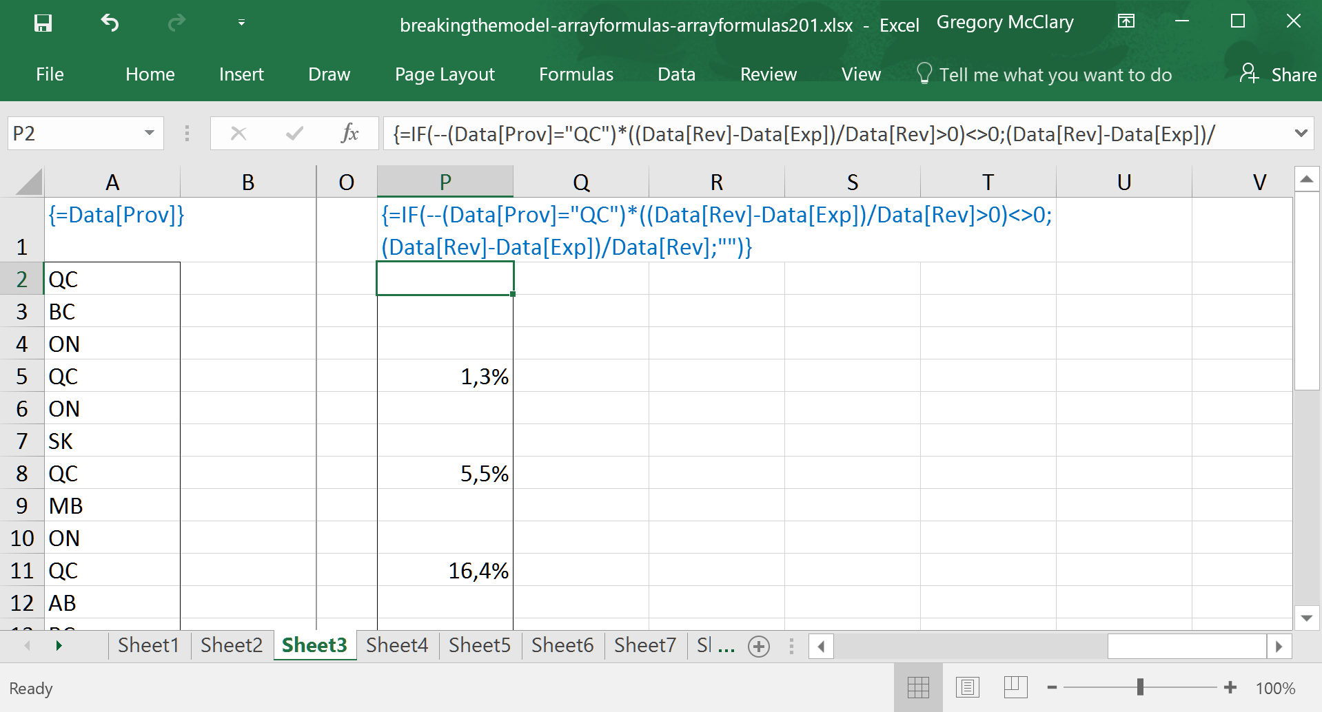
In this example, you will see (aside from the use of semi-colons instead of commas) that I’ve set up a multi-cell array formula to test whether each company is situated in Quebec. This shows a useful feature of the IF() function – that is, to conditionally replace data in a range with a desired value.
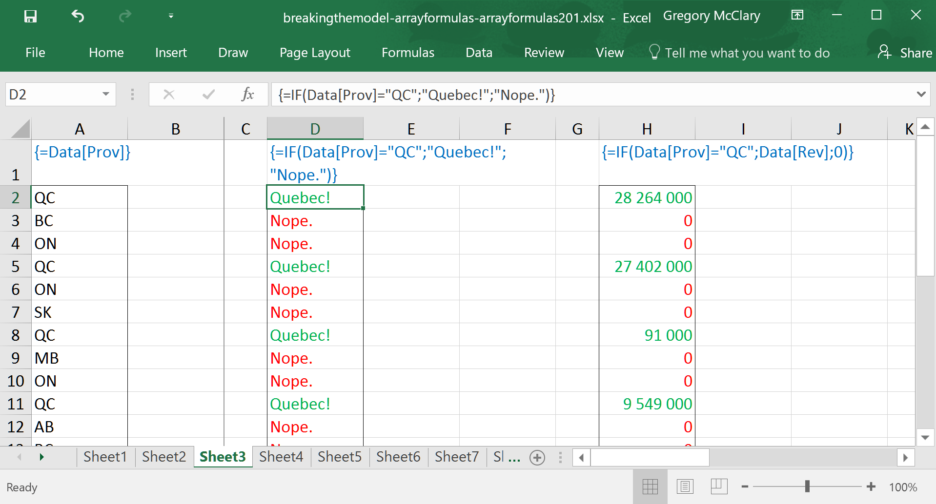
Here, we see a combination: if a company is in Quebec, the IF() formula returns the corresponding value from the revenue column; if not, it returns a zero.
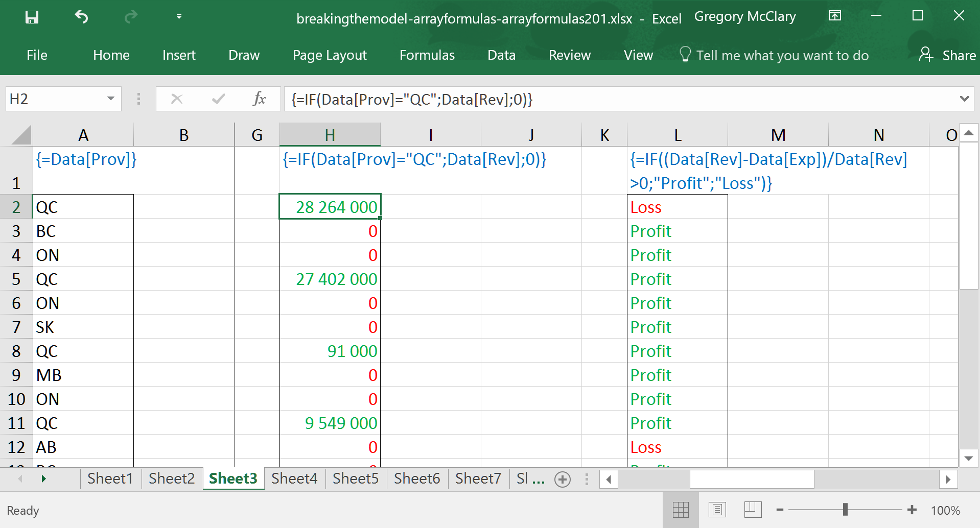
Importantly, Excel observes order of operations such that formulas are calculated after operations on ranges – in this case, Excel calculates profit margins for each company and then passes the array to the logical_test in IF(). The function then operates on each value and returns the specified text values.
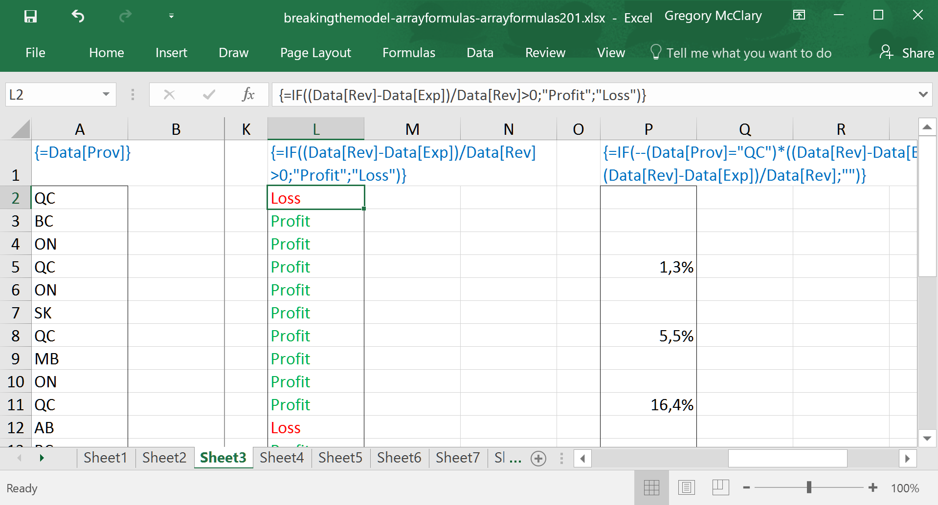
Finally, I’ve set up a slightly more interesting formula to illustrate where we’ll be heading in the next lesson. The ––()*()<>0 structure is explained in a bit; suffice to say that it’s the array formula equivalent of the AND() function. And to make it doubly odd, you can see that the results, when displayed in French, use commas instead of the usual decimal dots.
This formula tests for companies in Quebec that are profitable. Note also that it mixes the types of data that it returns. That is, if the conditions are both true, IF() returns the numerical profit margin of the company; otherwise, it returns a null text value.
So… this clearly presents some interesting possibilities, but beware – logical operations, and the resulting logical values (TRUE and FALSE) are handled a bit strangely in Excel. The following lesson will pick apart the logical operations that drive IF(), and thus lay the critical foundation for using this formula with confidence in the context of array formulas.
Lesson 4: Overly literal logical operations
So… array formulas are already a little bit awkward, and logical operations are where you’ll likely spend the bulk of your troubleshooting time. The following toggles outline the peculiarities associated with the logical operations that you use to control IF()’s behaviour.
The formula in column A is shown for convenience – this column of data is referenced in each of this lesson’s ‘steps’.
Shifting our gaze to column D, the formula tests if each company’s revenues are over $1,000,000. The first thing to notice is that Excel returns values of TRUE and FALSE when performing a logical operation (e.g. =, >, <, >=, <=, <>). There are also a few functions that return this type of value (e.g. ISERROR(), ISNUMBER(), etc.). Someday, I’ll compile a list of them and pontificate at length. In Excel parlance, this type of data is referred to as ‘logical’ values, and it is stored (and operated on) as a distinct type of data (e.g. numbers, dates, text, logical).
Note that logical operators are actually treated very similarly to mathematical operations – prepare to embrace the awkwardness of BEDMASL. As we’re all well aware, Excel respects the order of operations such that operations enclosed in Brackets are performed first, then Exponents, followed by Division, Multiplication, Addition, and Subtraction. Logical operations happen last, and they return logical values. Not numbers.
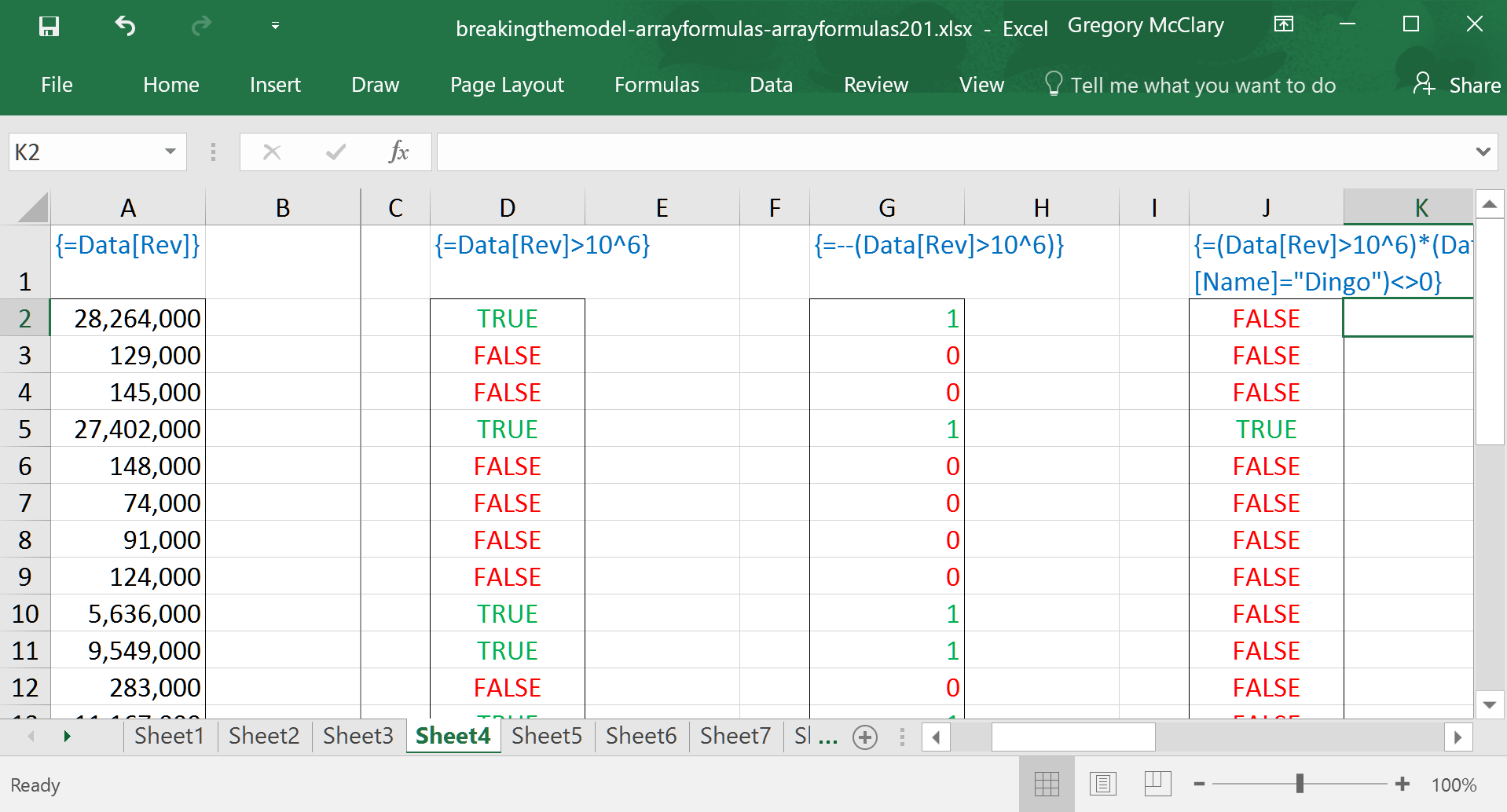
If we were really sneaky, we might find it useful for a logical operation to return 1 or 0 based on a logical operation. Look no further. If you perform a mathematical operation on a logical value, it behaves as though TRUE=1 and FALSE=0. In this case, I’ve invoked what I call the double negative (it’s got a real name, too: it’s a double unary operator). Mine’s less weird.
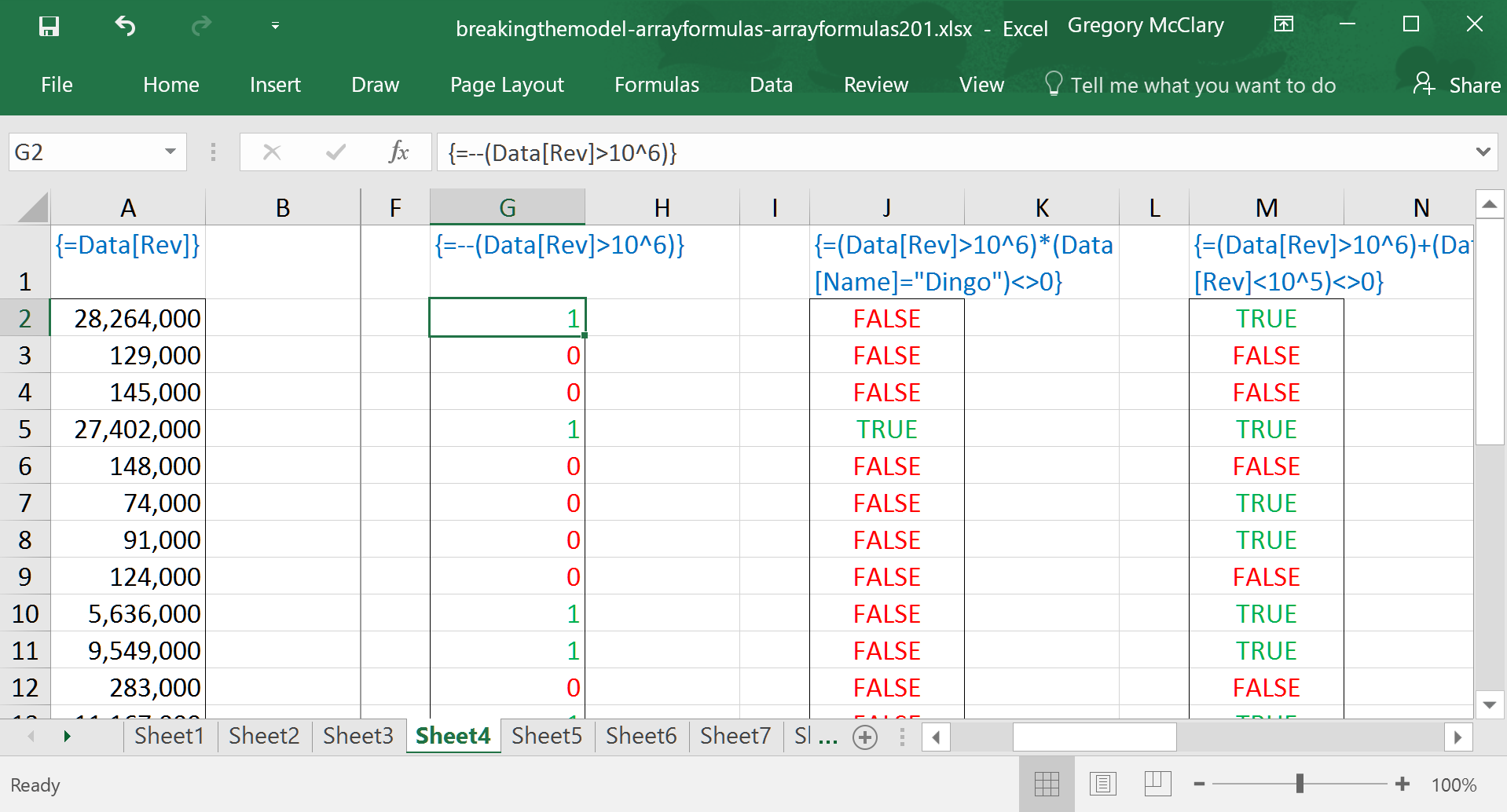
So what happens if we want to use an AND() function as part of a logical test? No dice.
It is, of course possible to achieve the intended result, but you have to get your hands a bit dirty to get there. The screenshot below shows how to use arithmetic, with an eye on order of operations, to create the intended result. Although arbitrary, I like to use <>0 to conclude expressions because it can also be used with a similar workaround for OR().
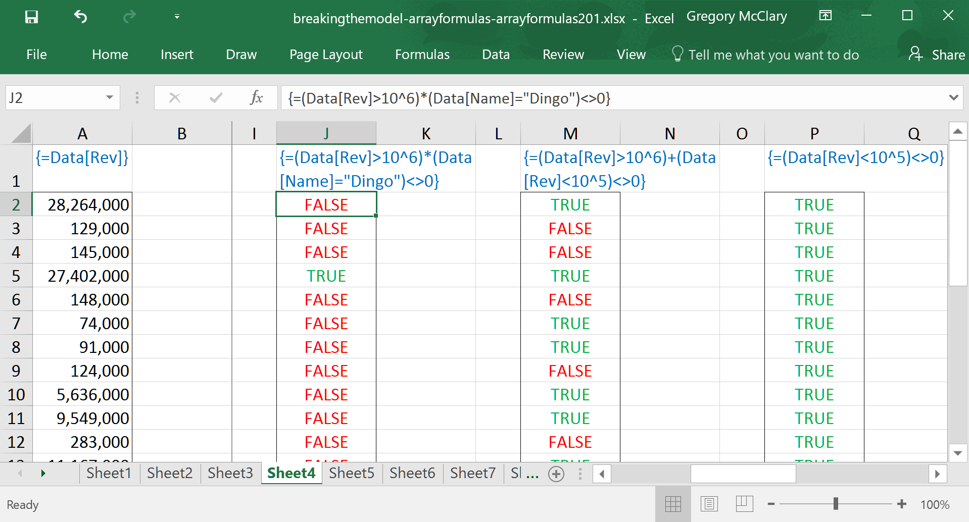
This formula shows that using addition, instead of multiplication, converts the ‘and’ expression into an ‘or’ condition. These can be applied in any combination you see fit to construct.
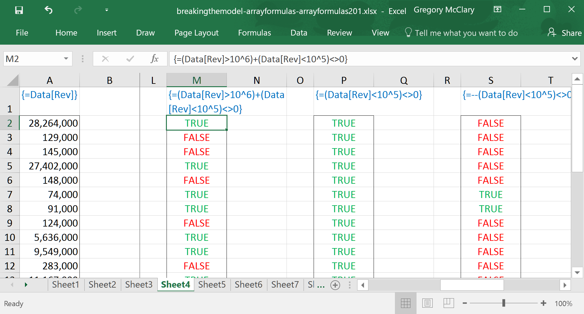
So… now begins the cautionary part of the tale. This formula asks Excel to evaluate whether the value returned by a logical expression is not equal to zero. Logical operators are different from mathematical operators in that they do not automatically translate logical values into 1 or 0. When Excel tests whether a value of FALSE is not equal to zero, it returns TRUE, because FALSE is, in fact, not equal to zero.
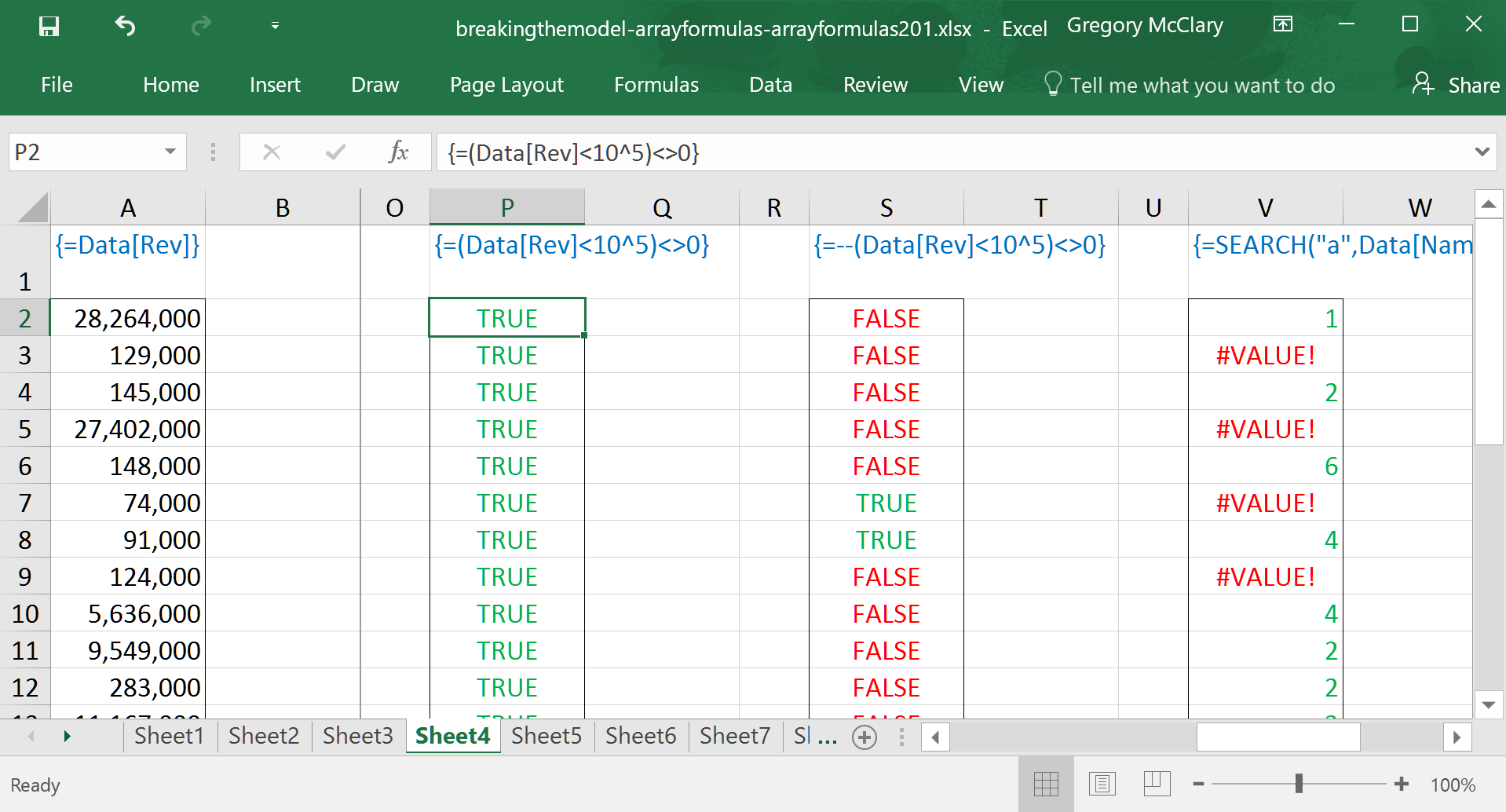
Here, I’ve solved the problem illustrated in the previous step. Using the double negative structure allows you to add and remove logical tests at will, without worrying about the formula breaking if you happen to delete all but one logical expression.
For anyone as paranoid as me about data integrity, I recommend using the full expression whenever implementing arithmetic-based logical operations:
––(logical_test1)*(logical_test2)<>0
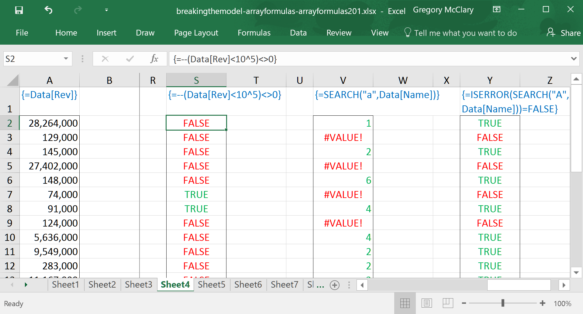
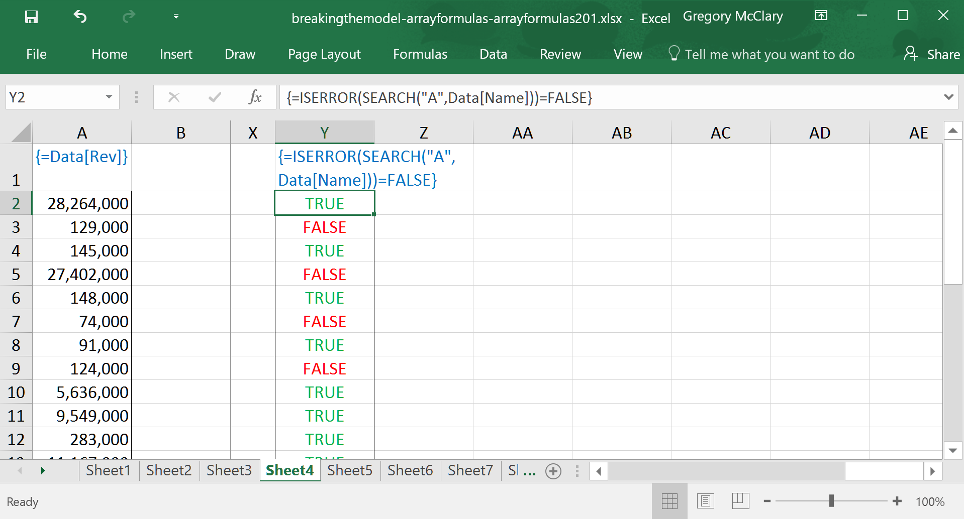
While we’re on the topic of Excel behaving weirdly, check this out – for some reason, Excel’s SEARCH() function returns an error if it does not find a match for your search term in the search text.
Not only is this annoying, it can be difficult to figure out where, in a more complex single-cell array formula, an error might originate. Always keep an eye out for functions that have behaviours that can push unwelcome surprises (errors) into the results of array calculations.
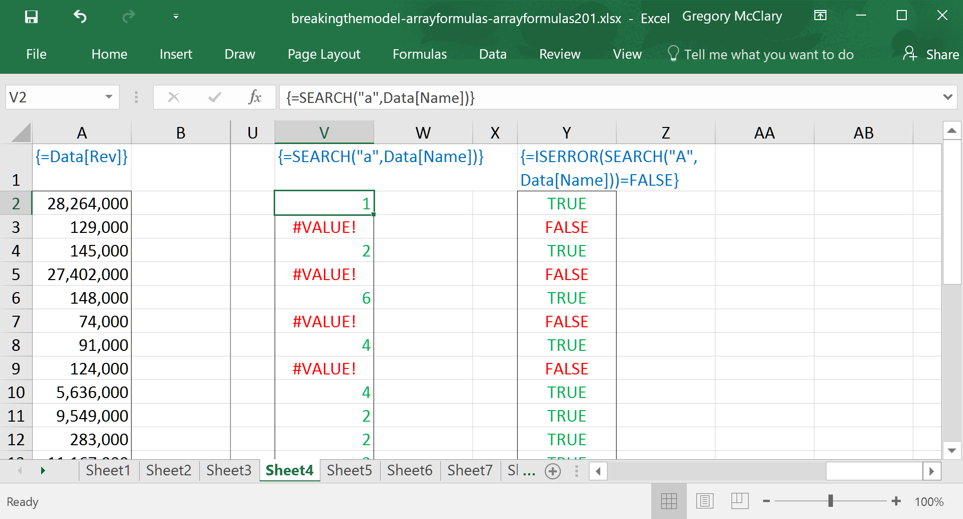
However, there is virtually always a way. In combination with an IF() function, this logical expression can be used to catch errors and prevent them from being passed on to another function/operation/formula.
After that lengthy preamble (Yes. That was a preamble.), we are now ready to pick up where Array Formulas 101 left off.
With that conceptual foundation in place, there’s a lot you can do. The following lesson looks at a few different ways we can use array formulas to broaden the scope of an analysis – the options are virtually limitless once these formulas begin to feel familiar.
Lesson 5: A mathemagical utopia, laden with choice
Let’s take a look at the implications of filtering when using single-cell array formulas.
As noted in Array Formulas 101, single cell array formulas are fabulous at retrieving descriptive statistics based on ranges of data – in particular, array formulas’ ability to control the order of operations gives you considerably more flexibility when calculating averages or any other summary descriptive statistic on a range of data. This example should serve as a reminder of (and slightly broader look at) the possibilities that were highlighted at the close of the previous article.
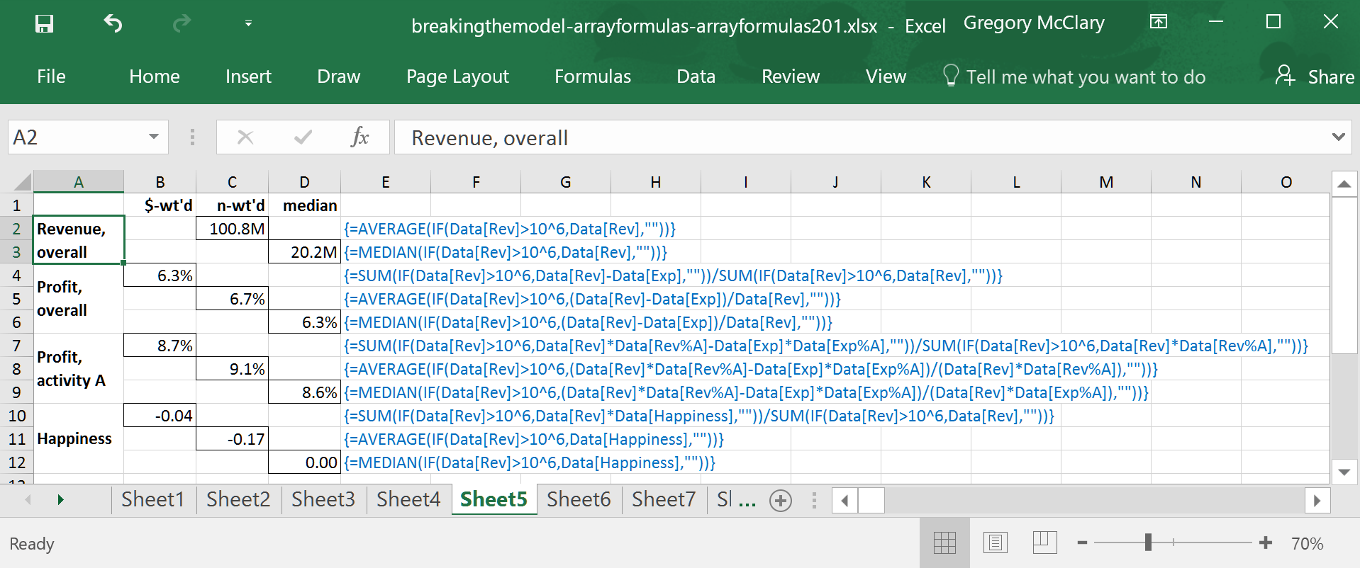
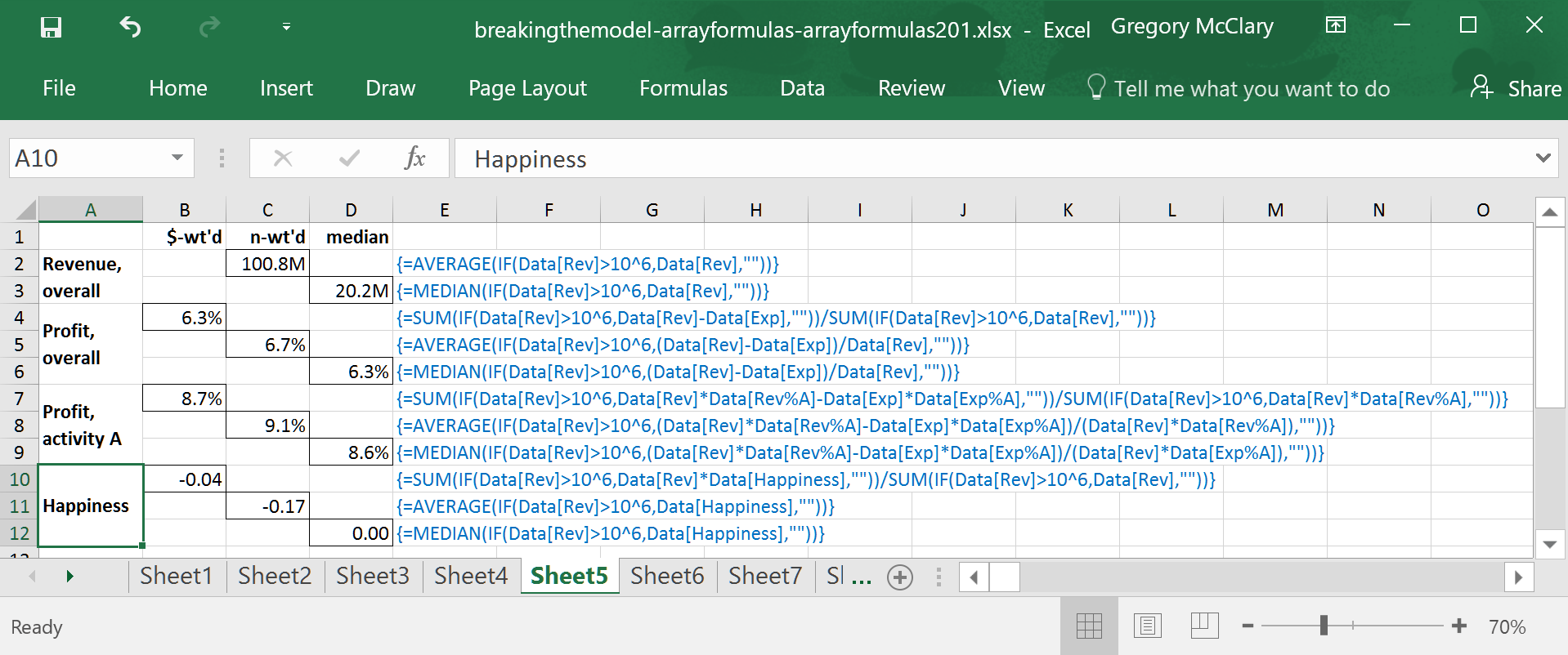
The examples in the screenshots below are organized by the focus of the analysis (column A), and the type of statistic (row 1). The formulas shown here were designed to illustrate some of the options on the table. All examples focus on the set of companies that make more than $1 million in revenue.
The first example just takes a quick look at revenues for companies that make more than $1 million. It bears repeating (from a passing mention in Array Formulas 101) that statistical functions in Excel ignore any text (or blank) values in the ranges that they operate on. Because IF() returns “” (specified in the value_if_false parameter), this formula performs exactly the same function as a filter in a pivot table.
The next few examples show a couple of ways that you could compute averages in an analysis of profitability.
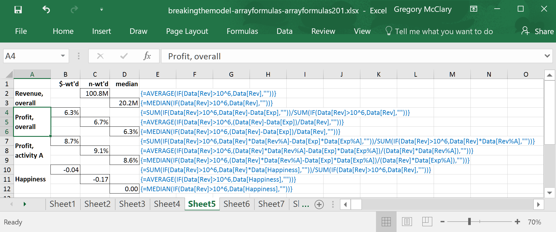
The formula in row 4 takes the total profit for the entire filtered sample and divides by the total revenue. This gives a profit margin for the sample as a whole, ignoring whether or not revenue tends to be concentrated among a few companies or widely distributed within the sample.
The formula in row 5 calculates average profitability on a company-by-company basis, regardless of the volume of sales at any one company. The difference between this and the previous calculation already tells us that companies with more sales volume are slightly less profitable than their smaller counterparts.
The formula in row 6 calculates the median in this sample – note that this formula is identical to the one that precedes it, replacing only the enclosing AVERAGE() with MEDIAN().
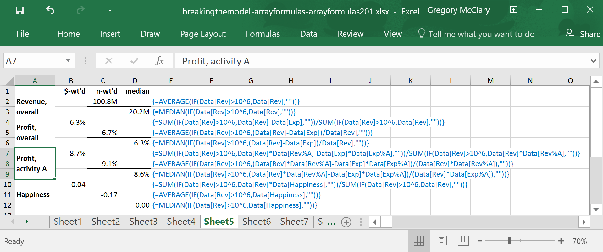
The example in row 7 is similar to the formula immediately above it in column B, except that it multiplies revenue and expenses by the percentage of each that relate to activity A. The result is the overall profitability of activity A within the sample as a whole.
Using a similar calculation to that appearing in row 5, the formula in row 8 finds an n-weighted average on a per company basis.
The formula in row 9 is, like the one above it, identical to the preceding example except for the enclosing MEDIAN().
The final set of examples are a little more interesting. While profitability is naturally weighted by the sales volumes of companies when calculated in aggregate, it requires a bit of manipulation to weight happiness in proportion to revenue. In this formula, happiness is multiplied by the total revenues at each company, and the total is divided by total revenues for the sample (thereby cancelling out the revenue factored into the numerator).
Used in tandem with a revenue-weighted average (as in row 10), this alternative weighting scheme gives insight into the distribution of happiness by profitability. For example, the disparity between this and the n-weighted average suggests that companies with more revenue are slightly less happy than the overall average. A quick comparison such as this may be a good indicator of whether a deeper analysis is a worthwhile pursuit.
Once again, the filter used to calculate the median in row 12 is identical to the formula that precedes it.
Filtering is all well and good, but it takes one more step to really reap the time savings and flexibility afforded by array formulas. The key ingredient, which became apparent to me only after a fair amount of trial and error, reduces to a few organizing principles. There is one final piece in the puzzle – LOOKUP().
There are some functions that are not available in array formulas. The technical nitty-gritty will be covered later in this series, but for the time being, prepare to embrace the LOOKUP() function. I’d never heard of this function until I started using array formulas, which don’t support the better known VLOOKUP(), HLOOKUP(), or INDEX(MATCH()), and found this capability useful enough to require it on a fairly regular basis.
While LOOKUP() works marvelously when used correctly (as demonstrated in the following examples), it can be a little finicky. Click the button below for a full rundown of LOOKUP(). Note that this site uses blue buttons to identify functions that might be useful, but are not recommended for general use due to limited functionality. Array Formulas 301 discusses INDEX(MATCH()), the preferred lookup formula for general use.
Use if necessary: Looks up tabulated data based on row headings – data must be sorted.
Joins text end-to-end
The remaining lessons in this article develop a versatile set of organizational principles that I would employ to conduct an efficient and systematic analysis of the data set that we’ve been working with throughout this article.
In the example here, I’ve just performed a ‘freestyle’ analysis to demonstrate some concepts, all of which take advantage of LOOKUP(). Note that I’ve used named tables to enclose any definitions that will be carried through the subsequent analysis. The following example is the focus of the remaining three lessons in this article. Broadly, the examples also show some interesting ways that one might use data to mine meaningful results from a large data set, culminating with a foray into cross tabulation.
Before we launch into the details, take a scroll through the overall design. This approach is an effective and intuitive way to mine survey data. It boasts the advantage of using definitions (in the locked pane on the left), which are referred to throughout the ensuing analysis. Should I wish to make a change in any assumption/definition/etc. later in the process, it will be a quick and easy edit.
In this case, I’ve organized my work by lining up all analysis that relates to a particular definition along rows. If you’re performing the same operation across different slices of data (e.g., profitability by province, by company size, by happiness, etc.), and especially cross tabulations (e.g., every question in a survey needs to be broken out by gender of the respondent) it’s possible to use the top pane as well.
The following lessons work through each of the three sections in the preceding example, one section at a time.
Lesson 6: Practical aesthetics (rows 3-14)
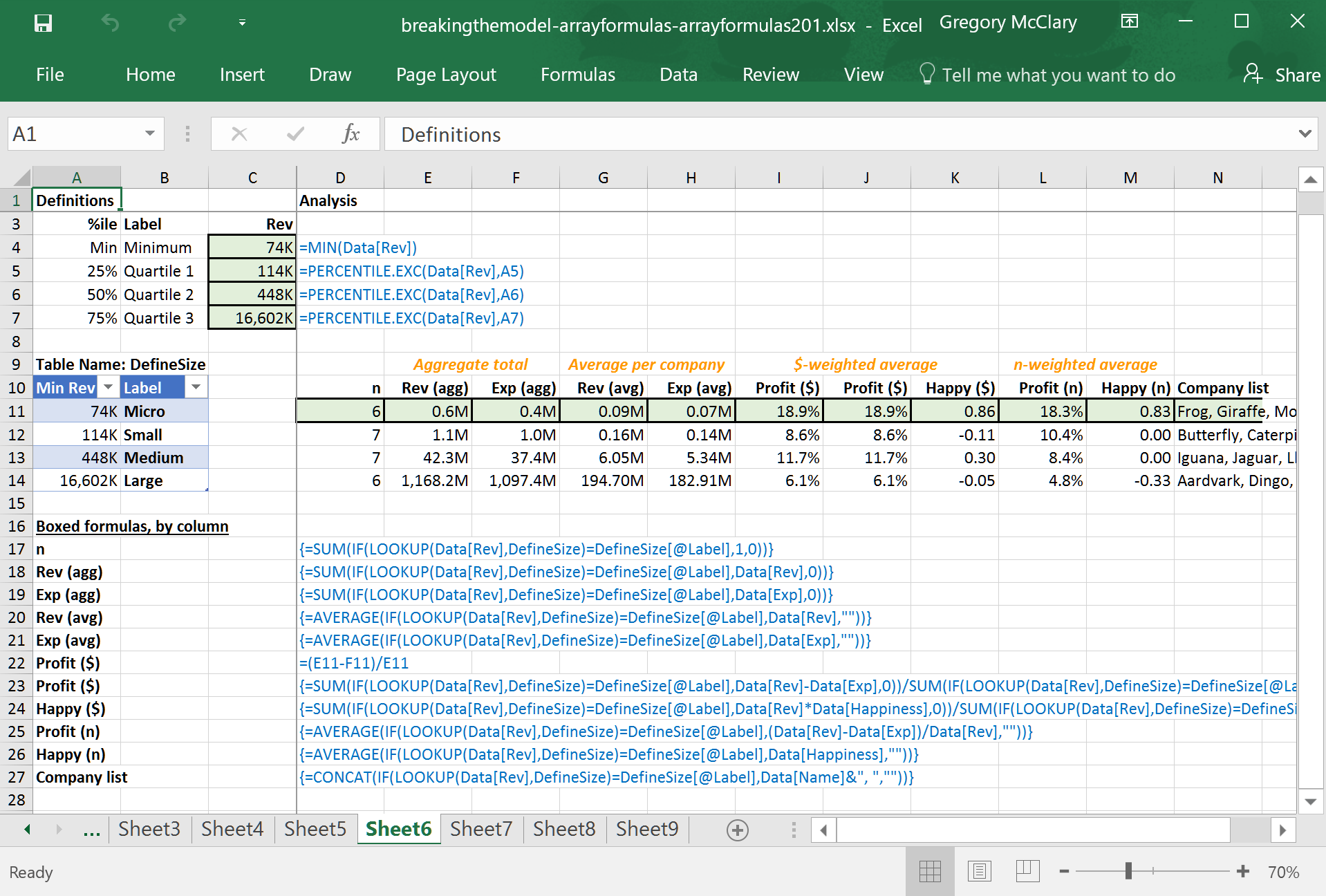
The screenshot below shows the formulas underlying rows 3-14. This set of rows illustrates the basic organizing principle used throughout this analysis.
Click the following toggles for a description of the elements used to construct the analysis.
Rows 3-7 in the ‘Definitions’ pane (columns A-C), use a few normal formulas to find revenue thresholds that are then used to define company size. I’ve performed this step separately because it leaves the door open to adjust the definitions later. For example, if I’m going to use this analysis to estimate industry size, I might need to incorporate a set of definitions that will exclude outliers and/or match the company sizes to whatever we end up using as a proxy for the distribution of company size in the industry ‘universe’.
Still focusing on the ‘Definitions’ pane (columns A-C), I’ve created a table that links to the revenue thresholds established in the preceding calculation. Note that the first column of this table must be sorted in ascending numerical/alphabetical/chronological order because LOOKUP() is the only lookup function that is compatible with array formulas and it will not work correctly with unsorted data.
The analysis that extends rightward from the locked pane filters data by company size using the LOOKUP() function. If you recall, the punchline in Lesson 3, Step 1 pointed out that the IF() function can be used to conditionally replace data with values as you see fit. LOOKUP() takes this capability one step farther by testing each value in our source column of data against the leftmost column in a lookup table (in this case, the table in the locked pane). The function then returns the corresponding value from the rightmost column.
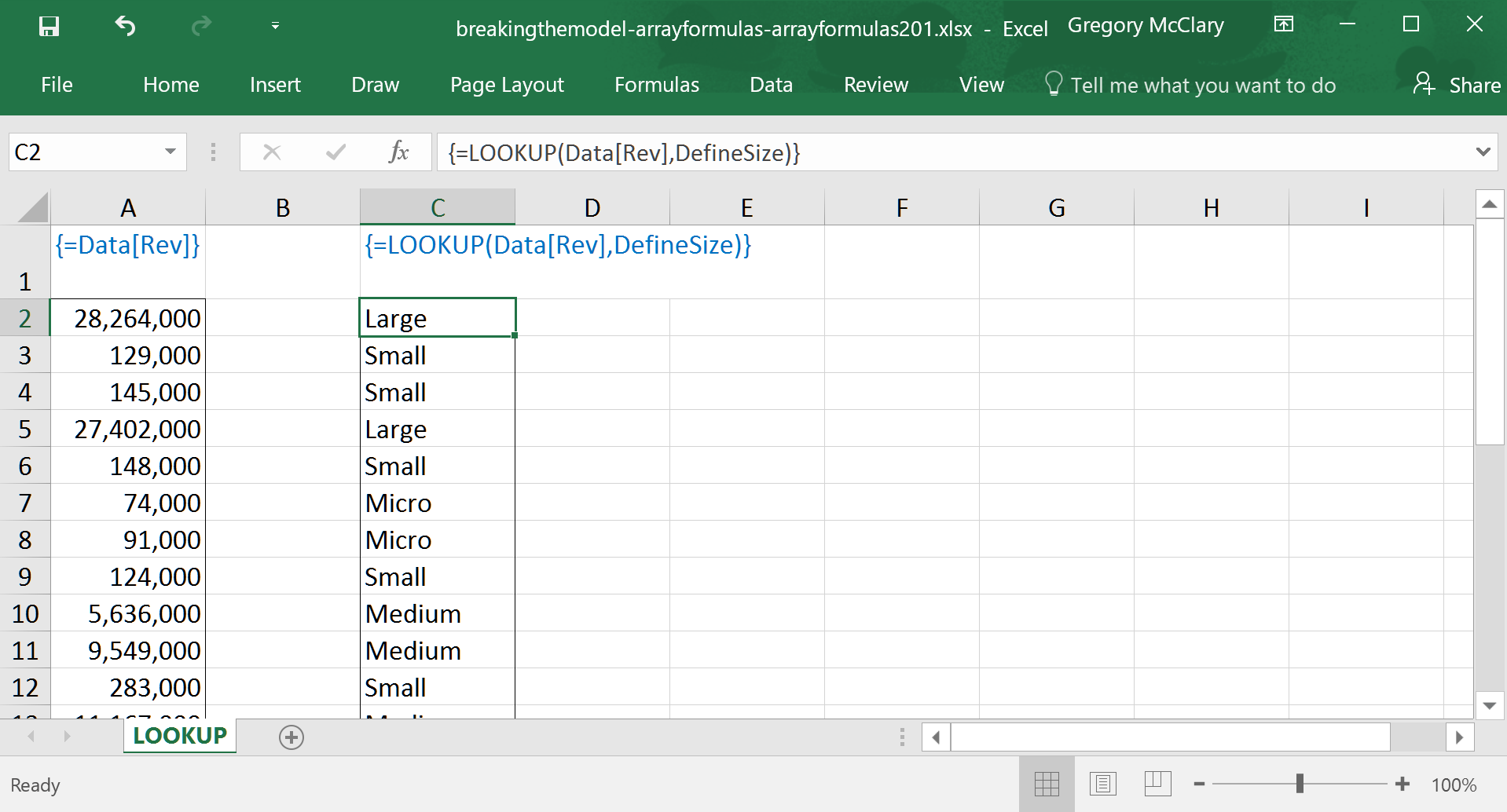
The screenshot below shows how Excel actually operates on a column of data using LOOKUP() and the company size definition table shown above. In the analysis above, the filter used in every formula to the right of the locked pane tests whether the result of the LOOKUP() function matches the value in the “Label” column in the same row.
This arrangement allows us to use the definition table labels twice – first, as the column from which LOOKUP() returns a value (as in the screenshot below); and second, it provides a value against which LOOKUP()’s result is tested. The benefit of using this approach is that if we ever need to add an extra row to the definitions, it’s just a matter of inserting a row, adding some new values in the definition table, and copying formulas down into the new row from the row above.
Apart from CONCAT(), which appears in column M, all of the functions used in this example were described earlier in this article.
The formula in column M shows how one might extract comma delimited lists from a data set. In this case, I’ve pulled the names of companies that are included in each size category. Returning lists can be extremely useful if your analysis requires that you identify data entries based on the same set of characteristics you’re using in a given row.
With all of this flexibility at your fingertips, array formulas can make your work more prone to error if you are not careful. This is particularly true when you need to revise previous work. Although it does take a bit of time and thought, there are a host of benefits that accompany the thorough use of sumchecks:
- First, when you set up a sumcheck, it forces you to find an alternative way to calculate a summary value. By performing these mental gymnastics, you will more quickly identify quirks in the data, which will support a more robust analysis and may inspire constructive follow-up inquiries.
- Second, finding efficient ways to check sums is a great way to discover new and interesting capabilities of array formulas.
- Third, by testing your work when it’s hot off the press (particularly if you’re new to array formulas), you will be more confident with your work.
- Finally, you can set up sumchecks that will help you identify any places where a future revision does not correctly flow through the model.
The following example introduces the use of sumchecks to automatically test whether the data you have retrieved is, in fact, complete and correct.
Lesson 7: Bring on the cross-tabs (rows 16-28)
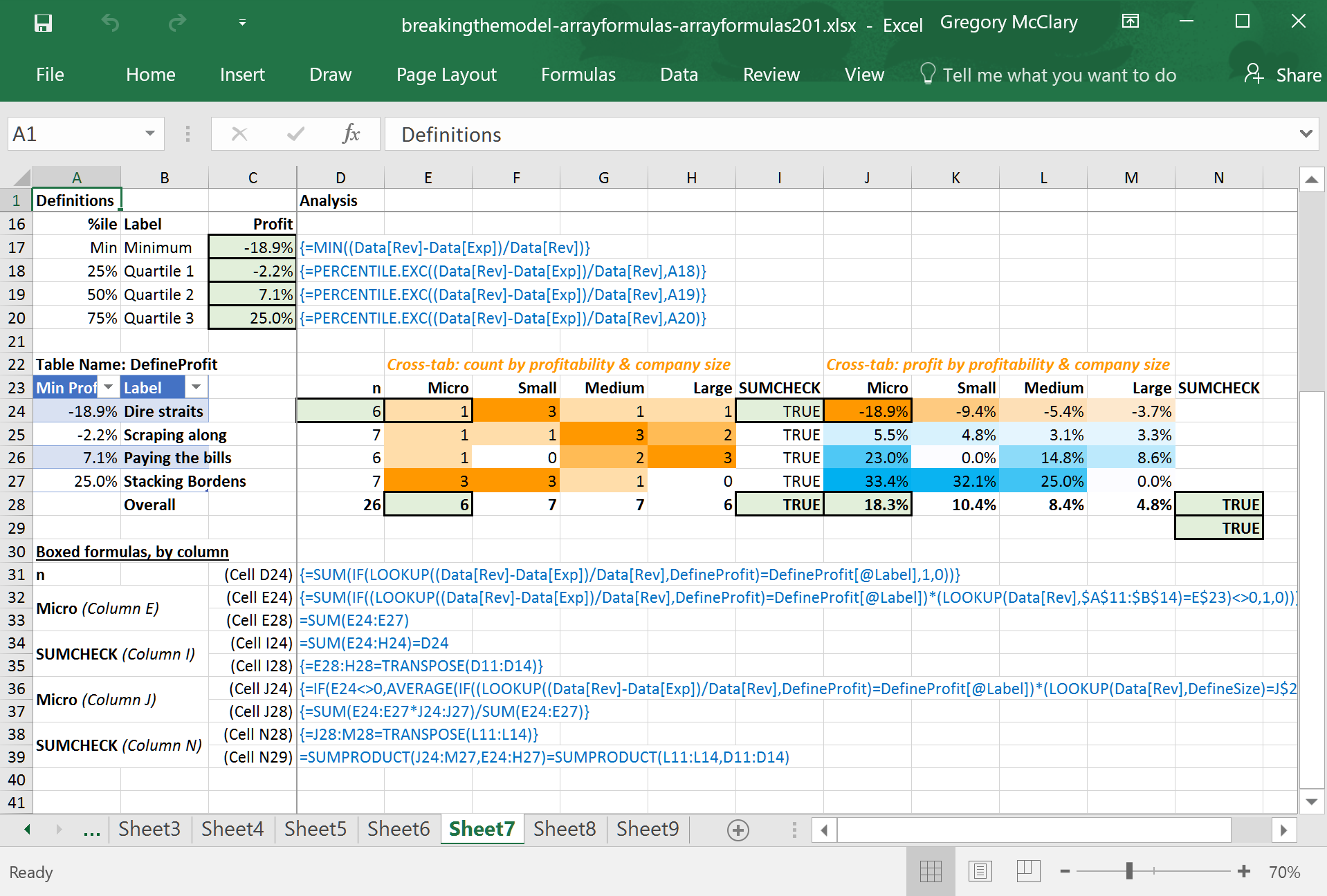
The screenshot below shows the formulas underlying rows 16-28. In this example, I’ve set up the formulas to cross-tabulate data in a couple of different ways. This approach has a couple of advantages over using pivot tables; you are completely in control of the layout, and you have discretion over which data is included and excluded from the result.
Note, however, that using array formulas to perform this function requires a little more care. For example, pivot tables automatically deal with blanks in the data pretty elegantly. When using array formulas, you have to keep track of whether a single-cell formula (or set thereof) is actually operating on and returning the values that you expect.
Click the following toggles to explore some of the ins and outs of implementing cross-tabs with array formulas.
As in the previous lesson, this example begins by setting up a definition. This time, I’ve calculated the thresholds that will be used to group companies by profitability. Unlike the previous example, this means that I need to calculate profitability for each company before calculating the percentile thresholds. As such, these formulas will only work if they are entered as array formulas.
In the ‘Definitions’ pane (columns A-C), this table is set up identically to the previous example. In this instance, I’ve added an ‘Overall’ row that can be used to perform sumchecks.
The first crosstab (column E) shows the distribution of companies by profitability and company size. The column headings are provided by a multi-cell array formula drawing values from the “Label” column in the company size definition table. In the crosstab formulas, I’ve added a second condition which tests company size for a match against these column headings. Voila! Crosstabs!
The second crosstab (column J) uses a formula that returns the n-weighted profitability, also filtered by profitability (based on the row headings) and company size (based on the column headings). This formula is essentially identical to that used for the first crosstab, except that the value_if_true parameter in the IF() function is set to return each company’s profitability instead of a 1, the value_if_false parameter is set to “” (to hide these values from AVERAGE()), and the enclosing function is AVERAGE() instead of SUM().
In both crosstabs, I’ve used conditional formatting to display the data as a heatmap for a quick visual inspection. It appears that the profitability of smaller companies varies more widely than that of large companies.
While the first sumcheck is pretty self-evident, the second crosstab in this portion of the analysis presents an interesting problem with regard to sumchecks. Now that I’m working with average profitability by segment, I’d like to make sure that the values I’m looking at can be reconciled with the n-weighted profitability that was calculated previously.
Here, the total row (referring to the formula in cell J28) calculates the n-weighted profitability of each column. The sumcheck in cell N28 uses an array formula to test that these values match the corresponding n-weighted average profit margins calculated in the previous section of the analysis. Likewise, the sumcheck in cell N29 condenses the same operation into one cell (i.e. eliminating the need for a ‘total’ row).
In some cases, you will encounter data that is not organized in a way that is conducive to your analysis. The following example shows how to group categorical data and reference columns in tables using the INDIRECT() function.
Returns the cell/range at the given cell address
This formula is extremely versatile, especially when used with tables to reference ranges of data.
Lesson 8: Other filtering operations (rows 30-46)
The screenshot below shows the formulas underlying rows 30-46. These cross-tabs use different definitional and data retrieval mechanisms than the previous examples. The first uses a table that associates categorical data (provinces) with groups (regions), and the second uses INDIRECT() to reference data that is distributed across a few columns in the source data table.
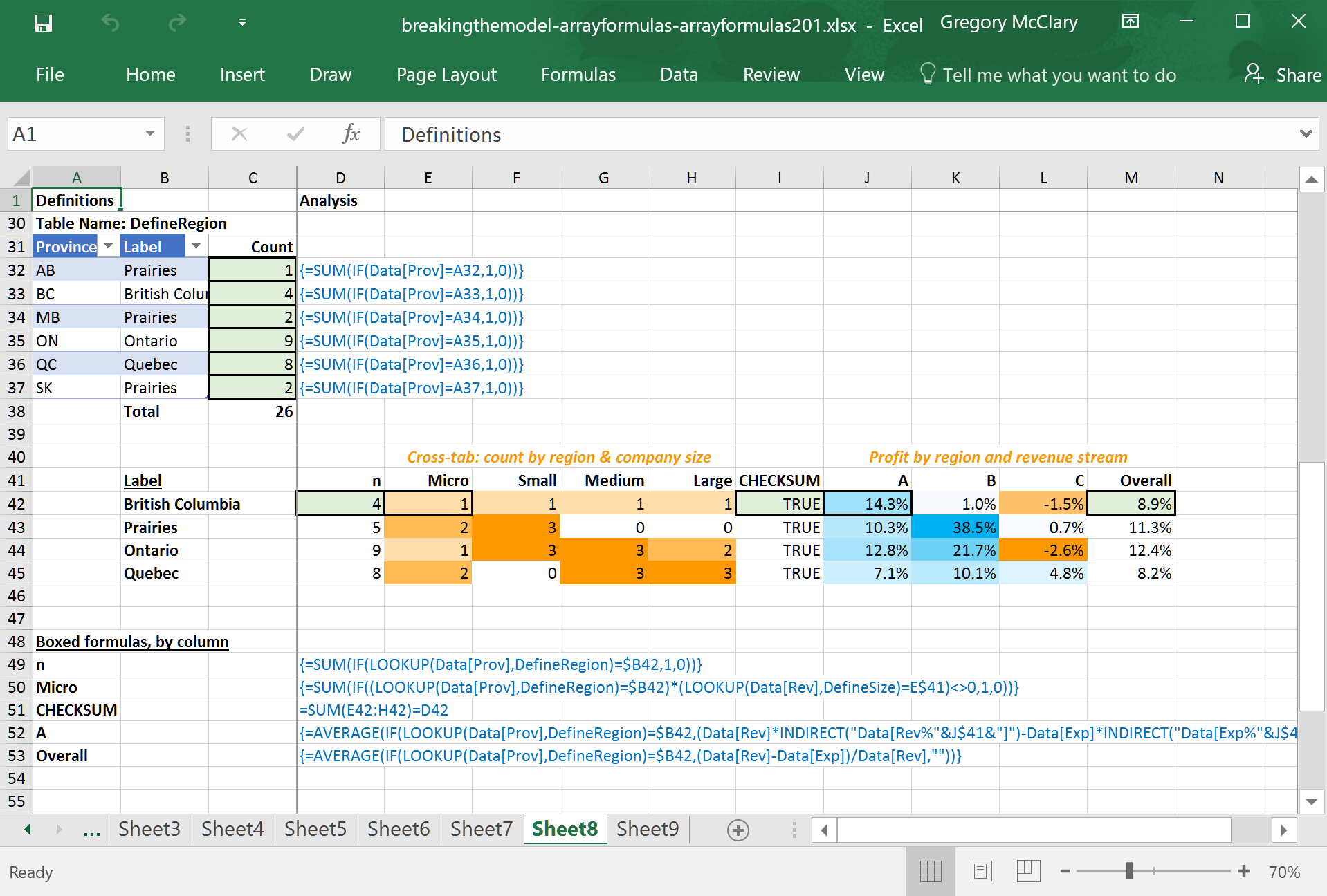
Click the following toggles for a description of the elements used to construct the analysis.
This section uses a slightly different mechanism than anything we’ve looked at thus far – in this case, the data contains the province in which the company is located. While Ontario and Quebec are significant (and distinct) regions, I would like to group the prairie provinces together because they have fewer respondents overall, and it’s silly to generalize about Alberta based on the response of one company. In order to group the provinces together, I set up an (alphabetically sorted) lookup table that returns the name of the region with which I want to associate each province.
The formulas in column C simply allow me to check how many companies reside within each province in the sample, to verify that each region will have a sufficiently large n-value.
Although this lone column of labels is less impressive than the previous lesson, note that this is a point where you will need to be careful. If you edit the definition table above, this list must be updated so that every region is included in the list.
To protect this sheet from accidental breakage, the sumcheck in cell D46 tests whether the total number of companies included for all regions matches the total number of companies calculated from all provinces. If there is a mismatch, the first thing to check would be whether your list of regions contains all of those defined in the table above.
Just like the preceding lesson, the first crosstab (in column E) adds a second filter that looks up the company size in the appropriate definition table and compares it to the column headings.
The final crosstab in this example is interesting. In this case, I have data on the percentage of total revenue derived from, and total expenses directed to, each of three revenue streams. At this point, I’m interested to compare the profitability of each revenue stream in the various regions. This is where things get interesting.
To keep my layout consistent, I’ve decided to use column headings to retrieve data from a relevant column. If you take a closer look at the formula, you’ll see that it filters by region, and then returns profitability computed such that: revenues (expenses) are multiplied by the percentage of revenues derived from (expenses directed to) the revenue stream identified in the column headings. The INDIRECT() function receives a concatenated string that identifies the table column corresponding to the crosstab column heading.
Epilogue
So… that covers what I consider to be one of the most useful applications of array formulas. Admittedly, I realize that this may be a lot to take in. There is definitely a bit of a learning curve on the road to array formula wizardry.
Stubbornness is a virtue.
If you can outlast this (often frustrating) break-in period, your future efficiency will be dazzling. My only advice at this point is to get out there and start finding opportunities to save yourself time. Array formulas 301 will continue in this spirit with ever more expansive applications in which you can use array formulas for virtually unlimited fun and profit.


